IEEE JOURNAL OF SOLID-STATE CIRCUITS, VOL. 48, NO. 6, JUNE 2013
1429
A 6-b 4.1-GS/s Flash ADC With Time-Domain Latch Interpolation in 90-nm CMOS Jong-In Kim, Ba-Ro-Saim Sung, Wan Kim, Member, IEEE, and Seung-Tak Ryu, Member, IEEE
Abstract—A 6-b 4.1-GS/s flash ADC was fabricated using a 90-nm CMOS with a time-domain latch interpolation technique that reduces the number of front-end dynamic comparators by half. The reduced number of comparators lowers power consumption, load capacitance to the T/H circuit, and the overhead of comparator calibration. The measured peak INL and DNL after comparator calibration are 0.74 and 0.49 LSB, respectively. The measured SNDR and SFDR are 31.2 and 38.3 dB, respectively, with a 2.02-GHz input at 4.1-GS/s operation while consuming 76 mW of total power. This ADC achieves a figure of merit of 0.625 pJ/conversion-step at 4.1 GS/s. Index Terms—Flash ADC, high-speed comparator, offset calibration, time-domain latch interpolation.
I. INTRODUCTION
W
ITH emerging applications such as ultra-wideband (UWB) and 60-GHz WPAN aiming at high data-rate communications, ADCs for these systems are requested to have several gigahertz-order sampling rates [1], [2]. One of the recent trends for such high-speed ADC design is interleaving low-power SAR ADCs [3]–[5]. However, various mismatches between the channels such as timing skew, offset, and gain error are very likely to degrade the performance and usually require complicated calibration schemes to overcome such issues. Traditionally, the most suitable ADC architecture for highspeed operation with low-to-medium resolution has been the flash type. However, preamplifiers, which are often required to relax the effects of comparator offset and metastability, increase the total power consumption. In addition, the input parasitic capacitance by the preamplifiers still remains a bottleneck for high-speed and low-power operation. One of the popular design techniques for addressing the above problem is the preamplifier interpolation scheme [6]–[8]. However, the static power consumption by the remaining preamplifiers is still not desirable given recent low power demand. Although the offset problem can be resolved without preamplifiers by using calibration [9]–[14], kickback noise from dynamic latches to the input signal (or sampling circuit) and to the reference ladder may degrade the signal integrity, resulting Manuscript received August 22, 2012; revised January 17, 2013; accepted February 05, 2013. Date of publication April 04, 2013; date of current version May 22, 2013. This work was supported by the National Research Foundation of Korea Grants funded by the Korean government (MEST) under Grant NRF2011-0006575 and Grant NRF-2012R1A2A2A01047062). This paper was approved by Associate Editor Lucien Breems. The authors are with KAIST, Daejeon, Korea (e-mail:
[email protected],
[email protected]). Color versions of one or more of the figures in this paper are available online at http://ieeexplore.ieee.org. Digital Object Identifier 10.1109/JSSC.2013.2252516
in SNR degradation. Thus, reduction of the number of dynamic latches will help to enhance the circuit performance by virtue of reduced dynamic noise. Recently, a time-domain latch interpolation technique that reduces the number of first-stage dynamic latches by half was proposed by the authors [14]. The present paper discusses detailed operational principles and design considerations of [14] and demonstrates an improved design with higher operating frequency and better performance. The remainder of this paper is organized as follows. The operational principle and the design considerations of the proposed time-domain latch interpolation technique are described in Section II. In Section III, the circuit implementation of a prototype 6-b flash ADC is presented. Section IV shows the experimental results, and Section V concludes the paper. II. TIME-DOMAIN LATCH INTERPOLATION TECHNIQUE A. Review of Preamplifier Interpolation (Voltage Domain, Linear Interpolation) Fig. 1(a) shows a schematic of the conventional voltage-domain preamplifier interpolation technique. It consists of preamplifiers of the first stage and two consecutive latch arrays (for high-speed decisions). After removing , whose output is shown as a dotted line, the missing information of the zero-crossing is generated (interpolated) by using the outputs from its neighboring stages, and , as shown in Fig. 1(b) illustrates. The input value where and crosses is the same zero-crossing point of the , and a virtual preamplifier ( ) is thus realized. Compared with the proposed latch interpolation technique discussed in Section II-B, the preamplifier interpolation can be understood as a voltage-domain linear interpolation where the interpolated output is a static function of a given input voltage, and the interpolated output divides the neighboring two zero-crossing points evenly (linearly). B. Time-Domain Latch Interpolation In order to distinguish the latch used as a comparator from the latch functioning as a pure digital storage element, the latch used for the comparator is hereafter referred to as a dynamic latch. Unlike the preamplifier, the dynamic latch is not a linear circuit for input voltage, because its output eventually reaches a logic high or low level depending only on the input polarity. Thus, linear voltage interpolation using the neighboring outputs at a steady state is not possible with dynamic latches. Nonetheless, the dynamic latch still shows input dependent nonsaturated
0018-9200/$31.00 © 2013 IEEE
1430
IEEE JOURNAL OF SOLID-STATE CIRCUITS, VOL. 48, NO. 6, JUNE 2013
Fig. 1. Conventional interpolation technique. (a) Architecture. (b) Transfer curve.
Fig. 2. Proposed time-domain latch interpolation technique. (a) Architecture. (b) Transient waveform.
behavior when it performs positive-feedback-based amplification, and, therefore, it is still possible to extract the interpolation information during a limited time period. The output settling behavior of a dynamic latch that is simply modeled as two cross-coupled inverters can be expressed as an exponential function with a time constant [15] as (1) where is the output voltage of the latch, is the initial output voltage at the beginning of the latching phase, is the transconductance of the inverter that incorporates the latch, and is the load capacitance. Equation (1) implies that the output settling behavior of a dynamic latch (before the output saturates) contains more than binary (low or high) information. A few recent studies showed that a single dynamic latch can achieve a resolution greater than 1 b by relying on this time-related information [16], [17]. However, since these techniques depend on the absolute timing, which is very sensitive to variations such as process, supply voltage, and temperature variations (PVT), background calibration must be used to map the timing information to certain voltage level(s). On the contrary, if the relative timing information between the latches can be used
for additional information, it will be robust to PVT variations. From (1) and [16], [17], we can expect that the outputs of two neighboring dynamic latches will show different input-dependent settling behaviors, even though they are not linear functions to the input. Fig. 2(a) shows the proposed time-domain latch interpolation technique. The structure has no preamplifier and is similar to that of the preamplifier interpolation technique shown in Fig. 1(a) in that a dynamic latch between and is eliminated from the first stage dynamic latch array. Dynamic latches are cascaded to compensate for insufficient latching time, as accomplished in many previous designs [7], [8], [14], [18]–[20], and those in the second array ( - ) amplify the outputs of the first-stage dynamic latches. Note that the circuits are drawn in a single-ended version for simplicity. Two dynamic latches and compare the input signal ( ) with their own references and , and the missing dynamic latch was supposed to compare with , where is the center level of and . The missing zero-crossing information by the eliminated dynamic latch is generated (interpolated) by in the second-stage dynamic latch array using two neighboring signals, and . Let us consider specific input cases in detail to understand the operational principle of the proposed technique. In Fig. 2(b),
KIM et al.: 6-B 4.1-GS/S FLASH ADC WITH TIME-DOMAIN LATCH INTERPOLATION IN 90-NM CMOS
Fig. 3.
–
1431
characteristics of two latches (a) without offset calibration and (b) with offset calibration.
the case where the input signal is located between and is shown as an example. The output waveforms of and are shown with the clock signal for the firststage dynamic latch array, CLK1. For the given input condition ( ), the input to , is positive and that to , is negative. then regenerates the positive output ( ) and ’s output becomes negative ( ). Since , the regeneration speed of is faster than that of , as (1) implies. As long as the output is in the transition period (before reaching the supply rails), the two adjacent dynamic latches, and , show an output level difference. The input waveform of the interpolation dynamic latch, ,( ) is shown in the figure. As long as the latching command for the second stage dynamic latch, CLK2, appears in a proper time range, can determine the polarity of the difference. As a result, the outputs of , , and are 1, 1, and 0, respectively. As another example, when , where , the dynamic latches in the first array operate oppositely to the case of , and , , and will produce 1, 0, and 0, respectively. As depicted in Fig. 2(b), the output interpolation of and is possible during a certain time period of : from when their outputs start to split to when they reach the supply rails. It is desirable to activate the second stage dynamic latch array when the interpolated signal ( ) is at roughly its peak value in order to overcome the offset of the following stage. Thus, the transition timing of CLK2 should be designed carefully (as described in the following section). Recently, a compact flash ADC with a latch-based interpolation technique that utilizes SR-latches as the second stage latches and does not require CLK2 was reported [21], and a patent similar to it could also be found [22]. Despite the convenience of CLK2-free latch interpolation in [21] and [22], it is not clear at what input condition (time and amplitude) the interpolation result is dominated in those techniques. Therefore, unlike the present work here, the accuracy of the interpolation result can possibly be degraded by the offsets of the following SR-latches unless they are designed carefully as if they are analog circuits. Detailed design considerations for the proposed latch interpolation scheme are discussed in the following Sections II-C and
III-C. Since the cascaded dynamic latches overcome the speed limitation of a single-stage dynamic latch, as briefly mentioned earlier, the proposed interpolation technique in the present work is not a burden in high-speed design where cascaded latches are required, especially under low supply voltage. C. Design Considerations for Time-Domain Latch Interpolation In applying the proposed time-domain latch interpolation technique, two kinds of mismatches in two neighboring dynamic latches must be considered: the input referred offset in each dynamic latch and the mismatch between the neighboring latches. Fig. 3(a) shows mismatched – characteristics of two input transistors in a dynamic latch. In order for the dynamic latch to determine zero-crossing information accurately, the dynamic latch offset should be sufficiently small, and, therefore, proper offset calibration should be performed, as shown in Fig. 3(b). However, in time-domain latch interpolation, interpolation using two offset calibrated dynamic latches does not always guarantee accurate zero crossing of the interpolated output even when the second stage latch’s offset is negligible. As can be inferred from Fig. 3(b), two offset cancelled dynamic latches are likely to have different values. If the values of the two dynamic latches are different, the output split times of the dynamic latches will be different for the same absolute input difference, as (1) implies. This results in a shift of the zero crossing point of the interpolated output. This phenomenon is illustrated in Fig. 4(a) and (b). Ideally, when the input is exactly at the center of and (i.e., ) and the dynamic latches are mismatch free, the output difference of must be always 0. However, here we consider a case where the of is larger than that of : . We simplify the problem by assuming well matched ’s in each dynamic latch. In this case, when , the transition of is faster than that of . Then, will identify that and shows equivalent decision error (equivalent offset in the eliminated virtual dynamic latch). A similar phenomenon can be found from the preamplifier interpolation case where an interpolation error
1432
IEEE JOURNAL OF SOLID-STATE CIRCUITS, VOL. 48, NO. 6, JUNE 2013
Fig. 4. Concept of input-referred offset due to the but .
mismatch in the first stage dynamic latches. (a) Test-bench. (b) Output waveform of the first latches when
Fig. 5. Block diagram of the prototype flash ADC.
occurs by the gain mismatches of the two neighboring preamplifiers [23]. More details on this are provided in the following section with an actual circuit design. III. PROTOTYPE FLASH ADC A prototype 6-b flash ADC has been designed utilizing the proposed latch interpolation technique. The overall structure of the ADC is shown in Fig. 5. The ADC consists of a
front-end track-and-hold amplifier (THA), a resistor ladder for reference generation, three stages of dynamic latches, a quasi-gray ROM-based encoder, calibration logics for the first stage dynamic latches, a clock buffer, and high-speed interfaces (LVDS) for the data and clock. The first-stage dynamic latch array is composed of 34 dynamic latches including dummies at both ends. 100- poly resistors are integrated on-chip for impedance matching at both the differential clock and the input terminals.
KIM et al.: 6-B 4.1-GS/S FLASH ADC WITH TIME-DOMAIN LATCH INTERPOLATION IN 90-NM CMOS
1433
Fig. 6. Track-and-hold amplifier.
A. Track-and-Hold Amplifier A THA is used to reduce the sampling error and the kickback noise from the first-stage dynamic latches. A schematic of the THA is shown in Fig. 6. The THA consists of nMOS sampling switches with dummy switches and a source follower. The differential input range of the ADC is 800 , while the input common mode voltage is set to 0.3 V. One least significant bit (LSB) is 12.5 mV. Since the maximum input level to the THA is as low as 0.5 V, no clock boosting was necessary for the nMOS sampling switches. The gate parasitic capacitance of the source follower and line parasitic are used for the hold capacitor. Considering a short sample time period of less than 125 ps at 4 GS/s operation, the transition time of the sampling clock has been reduced by locating the switch drivers (inverters in Fig. 6) close to the sampling switches. The dedicated supply voltage of the two inverters is shared with the THA in order to minimize sampling uncertainty from other digital blocks. Not only the clock paths but also the sampled signal paths from the THA to the dynamic latch array are carefully laid out considering the settling errors that depend on the dynamic latch locations. In the authors’ previous work [14], thin metal layers that have considerable parasitic resistance were used for the signal connection from the THA to dynamic latches. Consequently, even if the THA output was considered to be common to all of the following dynamic latches, the worst settling mismatch at the dynamic latch inputs was estimated to be about 15 mV at the instant of latching, and resulted in considerable performance degradation. Thus, in this design, the THA output is distributed to dynamic latches using the thickest metal lines given by the process, and the sampled voltage mismatch error is reduced to 0.3 mV. B. Dynamic Latch for the First Stage Fig. 7 presents the schematic of the dynamic latch designed for the use of the first-stage dynamic latch array. Compared with the widely used conventional structure [24], the dynamic latch for this work has an additional nMOS latch at the output to the ground path. This additional latch helps the dynamic latch to turn on rapidly from the reset phase by discharging the output node faster than in the conventional design, and it also reduces the latching delay. This characteristic yields another advantage, which is that the input transistor of the dynamic latch does not need to be increased for fast operation, unlike with the conventional designs. The proposed dynamic latch thus does not increase the capacitive load at the output of the THA and the
Fig. 7. Dynamic latch used for the first stage in this work.
Fig. 8. Simulated transient behaviors of the proposed and the conventional dynamic latches.
latching kickback is also not increased. Note that the input pair structure is simplified with a single differential pair while the real design for the first stage dynamic latches and the interpolation dynamic latches in the second stage have two differential pairs for differential input and references. Fig. 8 shows the simulation results of the conventional and the proposed dynamic latches. The proposed and conventional dynamic latches have the same sized transistors, and the only difference is the additional latch stage in the latter. The simulation was conducted at a 1.2-V supply voltage, 4-GHz clock frequency, and 1-mV input difference (about 0.1 LSB in our design) with 0.6-V input common voltage for the purpose of comparison. The simulation result shows enhanced latching speed compared with the conventional structure. The proposed scheme also has some drawbacks as well. The additional latch increases noise and offset level. This is not only due to the increased number of transistors, but also due to the effective gain reduction. Since the turn-on time of the dynamic latch is shortened due to the signal-independent fast discharge of the output via the additional NMOS latch to the ground, the contribution of the input signal to the output voltage difference is reduced when regeneration begins to dominate [25]. Because of this reduced effective gain, the input referred offset and noise increases. The input referred offset is slightly increased to 12.3 mV from the conventional one’s 10.7 mV . This offset problem is well compensated as will be discussed in Section III-C. The input referred noise of the proposed dynamic latch is about 1.15 mV while that of the conventional one
1434
IEEE JOURNAL OF SOLID-STATE CIRCUITS, VOL. 48, NO. 6, JUNE 2013
Fig. 9. Simplified calibration architecture and timing diagram.
is approximately 0.85 mV . Since the noise voltage corresponds to 0.1 LSB, the increased offset effect to the performance is not considerable. It should be noted that the reduced effective gain discussed here is focused only at the time when the regeneration begins and, therefore, it does not mean slow regeneration speed [recall in (1)]. As shown in Fig. 8, actual latching speed is enhanced because the total transconductance of the latches is increased due to the increased current through the pMOS and the increased total size of the nMOS. In addition, the regeneration operation begins earlier in the proposed design than it does in the conventional design. The dynamic latches in the second and the third stages have the conventional structure [24], because their latching time requirement is relaxed owing to the amplified signal via the first stage. C. Offset Calibration for First-Stage Dynamic Latches The accuracy of the proposed time-domain latch interpolation technique relies on low offset of the first dynamic latch array. Thus, the first-stage dynamic latches are calibrated and the body voltage control method has been used, similarly to several previously reported designs [3], [19]. Fig. 9 shows a block diagram of the offset calibration scheme and its timing diagram. The block diagram shows a single row of the three stages of dynamic latches and a simplified schematic of the first stage’s input pair. During the calibration mode, the inputs of the first-stage dynamic latches are disconnected from the THA and shorted to their own references. Depending on the third stage’s output, the body voltage is adjusted by proper switching to the resistor string. When the polarity of the third stage’s output changes, the control logic stops and the control word is stored in registers. Another important design point with the time-domain latch interpolation is the mismatch between the neighboring dynamic latches, as mentioned in Section II. Thus, using the designed dynamic latches, the input referred offset of the virtual
dynamic latch (for detection) induced by the mismatch problem has been verified, as shown in Fig. 10. Each dynamic latch is assumed to be offset-free, but the transistors in the dynamic latches and are sized differently with a certain error ratio in order for them to have mismatch. In detail, the values of and are adjusted in opposite directions in order to consider the worst case. The input-referred offset of the eliminated virtual dynamic latch can be found by sensing the output of . As we sweep the input slowly, the output of will flip at some point. The difference between that input level and is the equivalent input referred offset. The equivalent offset has been estimated by varying the amount of mismatch of the two dynamic latches. The values were estimated by assuming that the transistors are in the saturation region before the latching operation is completed. The standard deviation ( ) of the percentage mismatch was obtained from a Monte Carlo simulation and it revealed that 15% mismatch corresponds to error. Fig. 11 presents the mismatch-induced offset estimation results, which show that the value of the offset voltage is less than 1.25 mV for all process corners. Since this value is about 0.1 LSB of the designed ADC, the offset effect by the mismatch would not hurt performance. Temperature dependency of the mismatch was also simulated, but the effect was less signifiant than the corner variation. Owing to the large gain of the first stage dynamic latch, the dynamic latches in the second stage could be designed without need for offset calibration in this work. Fig. 12 shows the simulated input difference of the interpolating dynamic latch ( ), , at the rising edge of CLK2 as a function of the input difference between and , i.e., . When the input difference between and is 1 mV (about 0.1 LSB in the present design), is guaranteed to be more than 50 mV in all process corners. For this test, the time distance between CLK1 and CLK2 was set to 80 ps. Proper timing for CLK2 with respect to CLK1 is discussed in Section II-D.
KIM et al.: 6-B 4.1-GS/S FLASH ADC WITH TIME-DOMAIN LATCH INTERPOLATION IN 90-NM CMOS
Fig. 10. Test-bench for the input-referred offset by the
Fig. 11. Simulated input-referred offset by the dynamic latches ( and ).
mismatch of the first stage dynamic latches (
mismatch of the first stage
Fig. 12. Simulated output difference (input difference of the latch and . function of the input difference between
) as a
D. Clock Buffer and Clock Delay Circuit Fig. 13 shows a simplified schematic of the inverter-based clock buffers in the present work and the related timing diagram. For low switching noise, low-voltage differential signaling (LVDS) I/O [26] has been used. In order to reduce the load capacitance of the LVDS, three stages of cascaded inverters are used after LVDS, and then the first-stage dynamic latch clock (CLK1) is generated by using inverter delays. From CLK1, the THA clock (CLK_T), the second-stage dynamic
1435
and
).
latch clock (CLK2), and the digital logic clocks (CLK_D) are generated. CLK1 is buffered by two inverters, and the outputs of these inverters are applied to the THA clock. The accumulated RMS jitter of the sampling clock (CLK_T) by the five-stage inverter chain was estimated to be about 23 fs. This value was calculated from the phase-noise simulation result. Since the required RMS timing jitter for this ADC is 1 ps, the noise contribution by the five-stage inverter chain is negligible. Compared with our previous work [14], where CLK1 was generated by a delayed version of CLK_T, and hence a fixed short settling-time was given for the THA regardless of the sampling speed, we can derive the following advantages: since most of the time period of is used for the THA’s hold mode, the signal sampled by the THA can be transferred to every dynamic latch with enhanced settling accuracy (a time amount of only two inverter delays was sufficient for the hold time for the dynamic latches). The fixed two-inverter-delay time extends the THA settling time as the ADC sampling frequency is reduced. Thus, at lower speed, better ADC performance is guaranteed. As Fig. 2(b) illustrates, the clock edge distance between CLK1 and CLK2 is limited to the range of for proper time-domain latch interpolation. Note that it is important to set the time difference between CLK1 and CLK2 such that is maximized so that the effect of ’s offset will be negligible. From our simulation with all process corners, it was found that, as long as CLK2 follows CLK1 within a delay time range of 40 to 100 ps, (differential) was guaranteed to have more than 50 mV. In this design, the time spacing between CLK1 and CLK2 is controllable utilizing inverter delays with capacitor loads (clock delay circuit in Fig. 13). The clock buffer shown in Fig. 13 has been designed to guarantee that the time spacing between CLK1 and CLK2 lies in a range of 40–100 ps. Fig. 14 shows the simulation results. It is observed that all of the process corners with 2-b capacitor load control can satisfy the design requirements. When the temperature variation is also considered, the total range of time spacing between CLK1 and CLK2 is slightly extended as 43.6–117.8 ps across all corner variations. Note that this is the worst case estimation because the dynamic latches will experience the same process corner variation as the clock delay does, so more robust operation can
1436
IEEE JOURNAL OF SOLID-STATE CIRCUITS, VOL. 48, NO. 6, JUNE 2013
Fig. 13. Simplified clock buffer and clock delay circuit.
operational speed. By using a nonoverlap clock for the pull-up PMOS transistor of the first stage ROM, the shoot-through current in the pre-charge-based ROM is reduced. IV. MEASUREMENT RESULTS
Fig. 14. Simulated delay between CLK1 and CLK2 as a function of the decoder inputs (this simulation reflected supply bouncing due to the bond-wire inductance and other parasitic effects from the layout extraction).
be possible than the simulation showed. Deep n-well isolation is applied to the clock buffer and the LVDS to reduce noise coupling to the ADC core. E. ROM-Based Encoder A quasi-gray ROM-based encoder [8], [14], [18] was used for output code generation. In order to minimize the power consumption, we used nearly minimum-sized transistors for almost all logics. Each output node of the pre-charge-based ROM has one PMOS transistor (for pre-charge) and a number of NMOS transistors (for code generation). Since pre-charging of the output node using a single pMOS transistor can be very slow due to large parasitic capacitance at the node, the ROM has been divided into four sub-blocks, as shown in Fig. 15. This divided-by-four ROM structure in a 6-b flash ADC design gives the following advantages. First, as shown in Fig. 15(a), symmetrical routing is possible from the TSPC D flip-flop array to the ROM input, thus making the signal delay for each output even. Second, each output node of the divided ROM encoder has one PMOS transistor and eight nMOS transistors, and consequently all of the output nodes have exactly the same
A prototype chip was implemented in a nine-metal 90-nm CMOS process. A chip micrograph is shown in Fig. 16. The chip size, including all pads, is 2.5 1.1 mm and the active area of the ADC including the clock buffer is 0.38 mm , excluding I/Os and the calibration logic. The calibration logic designed for a functional proof of concept occupies considerable area (0.19 mm ), but the size can be reduced by sophisticated layout. The signal lines and power routing from the pads are routed using thick metal layers to reduce the parasitic resistance and more decoupling capacitors for the power supply could be buried under the high metal layer. Usually, a tree-structured signal connection is realized for signal and clock distribution when timing skew is critical; however, the long metal wires of the tree structure have significant parasitic resistance and result in considerable delay. Thus, in this design, straight thick metal lines that help to reduce parasitic resistance are used in critical signal paths in order to reduce the absolute delay time. Fig. 17 shows the measured differential nonlinearity (DNL) and integral nonlinearity (INL) using the sine-wave code density test method [27]. They are measured at 4.1 GS/s with an input frequency of 1.5 MHz. The measured peak DNL and INL without dynamic latch calibration are 1.6 and 2.79 LSB, respectively. With calibration, the peak DNL and INL are reduced to 0.49 LSB and 0.79 LSB, respectively. The robustness of the proposed time-domain interpolation scheme was also tested as we changed the supply voltage and the 2-b delay control code (shown in Fig. 13). Both INL and DNL stayed less than 1 LSB with a supply voltage ranging from 1.05 to 1.28 V. The performance change was negligible as we changed the clock delay control. This proves that the proposed time-domain latch interpolation scheme coupled with the body voltage calibration functions robustly without missing code or wide code.
KIM et al.: 6-B 4.1-GS/S FLASH ADC WITH TIME-DOMAIN LATCH INTERPOLATION IN 90-NM CMOS
1437
Fig. 15. Design issue of digital backend. (a) Routing and (b) block diagram of the ROM and circuit detail.
Fig. 16. Chip microphotograph.
Figs. 18 and 19 show the measured output spectrum for input frequencies of 2 MHz and 2.02 GHz at a 4.1-G/s sampling rate with and without the dynamic latch offset calibration. The output data were decimated by a factor of 64 considering the speed limitation of the data capture board. By utilizing the calibration, the SNDR of the ADC was improved from 25.7 and 25 dB to 33 and 31.2 dB at 2-MHz and 2.02-GHz input frequencies, respectively. The locations of the second and third harmonics are indicated by the numbers in Figs. 18 and 19. The dynamic performances with respect to input frequencies are shown in Fig. 20(a). With a low input frequency of 1 MHz, the ADC achieves a SNDR of 33.2 dB and a SFDR of 43.1 dB. With Nyquist input, the SNDR and SFDR are 31.2 and 38.3 dB, respectively. The sudden performance drop above 2-GHz input is from the characteristics of the signal source because proper filters could not be used for the input signals above that fre-
quency in our test. Fig. 20(b) plots the measured SNDR and SFDR as a function of the sampling frequency at a 450-MHz input frequency. The SNDR stays above 32 dB up to the conversion speed of 4.1 GS/s. Table I shows comparisons of the ADC in this work with several previously reported 5–8-b flash ADCs fabricated in the same technology node of 90-nm CMOS [8], [10], [13], [28], [29]. The ADC in the present work achieves competitive performance with the highest conversion speed and lowest FOM except for the 5-b design in [10]. Since the primary target of this work was a 60-GHz application requiring signal bandwidth of 1.728 GHz or higher, all of the circuit blocks were designed for more than 4-GS/s operation and, thus, the prototype does not show competitive FOM at low operating frequencies although the design has a slight static power consumption (370 W of static power by the resistor string for the reference generation).
1438
Fig. 17. Measured (a) DNL and (b) INL with and without calibration at
IEEE JOURNAL OF SOLID-STATE CIRCUITS, VOL. 48, NO. 6, JUNE 2013
1.5 MHz,
4.1 GS/s.
Fig. 18. Measured output spectrum (a) without calibration and (b) with calibration (
4.1 GS/s,
2 MHz).
Fig. 19. Measured output spectrum (a) without calibration and (b) with calibration (
4.1 GS/s,
2.02 GHz).
In order to compare the performance of our work with all 6-8-b ADCs with sample rates lower than 4.5 GS/s, their FOMs are plotted in Fig. 21. Few ADCs are found that can be applied for 60-GHz applications with sample rates over 3.5 GS/s other than those in [8], [30], and the present work. The prototype of this work shows the lowest FOM of 625 fJ/conversion-step among them. A 40-nm CMOS 3-GS/s flash ADC recently reported in [21] shows an excellent FOM by utilizing a similar but simpler operational principle of time-domain latch interpolation.
A summary of the presented ADC performance is provided in Table II. The total power consumption of the ADC core is 76 mW at a 4.1-GHz sampling rate, excluding I/Os. The dominant contributor to power consumption is the clock buffer, consuming 40% of the total power. Since the length of the flash ADC core was determined to be quite long (0.84 mm) by the input transistors of the first-stage dynamic latch, which use large-sized deep n-wells for body control, the long clock distribution leads to a heavy load of the clock buffer. Dis-
KIM et al.: 6-B 4.1-GS/S FLASH ADC WITH TIME-DOMAIN LATCH INTERPOLATION IN 90-NM CMOS
1439
Fig. 20. Measured SNDR/SFDR versus (a) input frequency at 4.1-GSample/s and (b) various conversion rates with a 450-MHz input.
Fig. 21. FOM for previously reported 6–8-b all-type ADCs and this work.
TABLE I PERFORMANCE COMPARISON (5–8-b FLASH ADCS IN 90-nm CMOS)
tributed clock buffering like clock-tree might have been better solution to reduce power overhead considering that jitter is not a concern here by virtue of the front-end THA. Alternatively, a size-efficient dynamic latch layout with a different offset calibration scheme (by avoiding a deep n-well) could have
reduced the clock driver power consumption. From the test, the dynamic latch was proved to be sufficiently fast for 4.1-GS/s operation owing to the cascaded dynamic latch array design. Instead, the maximum speed was limited by the digital backend, wherein most of the parts use the minimum-size transistors.
1440
IEEE JOURNAL OF SOLID-STATE CIRCUITS, VOL. 48, NO. 6, JUNE 2013
TABLE II PERFORMANCE SUMMARY
Thus, similar to previous works [31], [32], the supply voltage for the digital backend in this design was increased as the sample rate increased. The digital backend was tested with supply voltages of 0.9, 1.2, and 1.5 V at sample rates of 1, 2.5, and 4.1 GS/s, respectively. Excluding the parts of the digital backend, the other parts used a 1.2-V supply for the performance measurements. V. CONCLUSION This paper presents a 6-b 4.1-GS/s flash ADC using the proposed dynamic latch interpolation technique. By utilizing the input-dependent latching time difference between two neighboring dynamic latches, the interpolation function was successfully implemented. The proposed technique reduces the number of first-stage dynamic latches by half and thus reduces power consumption and hardware complexity. ACKNOWLEDGMENT The authors would like to thank the IDEC of KAIST for the CAD tools. REFERENCES [1] D. A. Sobel and R. W. Brodersen, “A 1 Gb/s mixed-signal baseband analog front-end for a 60 GHz wireless receiver,” IEEE J. Solid-State Circuits, vol. 44, no. 4, pp. 1281–1289, Apr. 2009. [2] S. Pinel, S. Sarkar, P. Sen, B. Perumana, D. Yeh, D. Dawn, and J. Laskar, “A 90 nm CMOS 60 GHz radio,” in IEEE Int. Solid State Circuits Conf. Dig. Tech. Papers, Feb. 2009, pp. 130–601. [3] E. Alpman, H. Lakdawala, L. R. Carley, and K. Soumyanath, “A 1.1 V 50 mW 2.5 GS/s 7 b time-interleaved C-2C SAR ADC in 45 nm LP digital CMOS,” in IEEE Int. Solid-State Circuits Conf. Dig. Tech. Papers, Feb. 2009, pp. 65–77. [4] C.-H. Chan, Y. Zhu, S.-W. Sin, S.-P. U, and R. P. Martins, “A 3.8 mW 8 b 1 GS/s 2 b/cycle interleaving SAR ADC with compact DAC structure,” in Dig. Symp. VLSI Circuits, 2012, pp. 86–87. [5] D. Stepanovic and B. Nikolic, “A 2.8 GS/s 44.6 mW time-interleaved ADC achieving 50.9 dB SNDR and 3 dB effective resolution bandwidth of 1.5 GHz in 65 nm CMOS,” in Dig. Symp. VLSI Circuits, 2012, pp. 84–85. [6] R. E. J. van de Grift, I. W. J. M. Rutten, and M. van der Veen, “An 8-bit video ADC incorporating folding and interpolation techniques,” IEEE J. Solid-State Circuits, vol. 22, no. 22, pp. 944–953, Dec. 1987. [7] K. Sushihara, H. Kimura, Y. Okamoto, K. Nishimura, and A. Matsuwasa, “A 6 b 800 MSample/s CMOS A/D converter,” in IEEE Int. Solid-State Circuits Conf. Dig. Tech. Papers., 2001, pp. 428–429.
[8] K. Deguchi, N. Suwa, M. Ito, T. Kumamoto, and T. Miki, “A 6-bit 3.5 GS/s 0.9-V 98-mW flash ADC in 90 nm CMOS,” IEEE J. Solid-State Circuits, vol. 43, no. 10, pp. 2303–2310, Oct. 2008. [9] G. van der Plas, S. Decoutere, and S. Donnay, “A 0.16 pJ/conversionstep 2.5 mW 1.25 GS/s 4 b ADC in a 90 nm digital CMOS process,” in IEEE Int. Solid-State Circuits Conf. Dig. Tech. Papers, Feb. 2006, pp. 566–567. [10] B. Verbruggen, P. Wambacq, M. Kuijk, and G. Van der Plas, “A 7.6 mW 1.75 GS/s 5 b flash A/D converter in 90 nm digital CMOS,” in Dig. Symp. VLSI Circuits, 2008, pp. 14–15. [11] H. Chung, A. Rylyakov, Z. T. Deniz, J. Bulzacchelli, G.-Y. Wei, and D. Friedman, “A 7.5-GS/s 3.8-ENOB 52-mW flash ADC with clock duty cycle control in 65 nm CMOS,” in Dig. Symp. VLSI Circuits, 2009, pp. 268–269. [12] G. Keskin, J. Proesel, J.-O. Plouchart, and L. Pileggi, “Exploiting combinatorial redundancy for offset calibration in flash ADCs,” IEEE J. Solid-State Circuits, vol. 46, no. 8, pp. 1904–1918, Aug. 2011. [13] J. Pernillo and M. Flynn, “A 1.5 GS/s flash ADC with 57.7 dB SFDR and 6.4 bit ENOB in 90 nm digital CMOS,” IEEE Trans. Circuits Syst. II, Exp. Briefs, vol. 58, no. 12, pp. 837–841, Dec. 2011. [14] J.-I. Kim, W. Kim, B. Sung, and S.-T. Ryu, “A time-domain latch interpolation technique for low power flash ADCs,” in Proc. IEEE Custom Integr.Circuits Conf., 2011, pp. 1–4. [15] B. Razavi, Principles of Data Conversion System Design. New York, NY, USA: IEEE Press, 1995. [16] A. Shikata, R. Sekimoto, T. Kuroda, and H. Ishikuro, “A 0.5 V 1.1 MS/sec 6.3 fJ/conversion-step SAR-ADC with tri-level comparator in 40 nm CMOS,” IEEE J. Solid-State Circuits, vol. 47, no. 4, pp. 1022–1030, Apr. 2012. [17] J. Guerber, H. Venkatram, M. Gande, A. Waters, and U. Moon, “A 10-b ternary SAR ADC with quantization time information utilization,” IEEE J. Solid-State Circuits, vol. 47, no. 11, pp. 2604–2613, Nov. 2012. [18] M. Choi and A. A. Abidi, “A 6-b 1.3-Gsample/s A/D converter in 0.35 m CMOS,” IEEE J. Solid-State Circuits, vol. 36, no. 12, pp. 1847–1858, Dec. 2001. [19] J. Yao, J. Liu, and H. Lee, “Bulk voltage trimming offset calibration for high-speed flash ADCs,” IEEE Trans. Circuits Syst. II, Exp. Briefs, vol. 57, pp. 101–114, Feb. 2010. [20] S. Sheikhaei, S. Mirabbasi, and A. Ivanov, “A 43 mW single-channel CMOS,” in Proc. IEEE Custom 4 GS/s 4-bit flash ADC in 0.18 Integr.Circuits Conf., Sep. 2007, pp. 333–336. [21] Y.-S. Shu, “A 6 b 3 GS/s 11 mW fully dynamic flash ADC in 40 nm CMOS with reduced number of comparators,” in Dig. Symp. VLSI Circuits, 2012, pp. 26–27. [22] M. Waltari, “Time Domain Interplation Scheme for Flash A/D Converters,” U.S. Patent 7 557 746, Jul. 7, 2009. [23] M. Choe, B. Song, and K. Bacrania, “A 13 b 40 MS/s CMOS pipelined folding ADC with background offset trimming,” IEEE J. Solid-State Circuits, vol. 35, no. 12, pp. 1781–1790, Dec. 2000. [24] B. Wicht, T. Nirschl, and D. Schmitt-Landsiedel, “Yield and speed optimization of a latch-type voltage sense amplifier,” IEEE J. Solid-State Circuits, vol. 39, no. 7, pp. 1148–1158, Jul. 2004. [25] D. Schinkel, E. Mensink, E. Klumperink, E. Van Tuijl, and B. Nauta, “A double-tail latch-type voltage sense amplifier with 18 ps Setup+Hold time,” in IEEE Int. Solid-State Circuits Conf. Dig. Tech. Papers, Feb. 2007, pp. 314–315. [26] A. Boni, A. Pierazzi, and D. Vecchi, “LVDS I/O Interface for Gb/sCMOS,” IEEE J. Solid-State Circuits, per-pin Operation in 0.35 vol. 36, no. 4, pp. 706–711, Apr. 2001. [27] J. Doemberg, H.-S. Lee, and D. A. Hodges, “Full-speed testing of A/D converters,” IEEE J. Solid-State Circuits, vol. SC-19, no. 6, pp. 820–827, Dec. 1984. [28] H. Yu and M.-C. F. Chang, “A 1-V 1.25-GS/S 8-bit self-calibrated Flash ADC in 90-nm digital CMOS,” IEEE Trans. Circuits Syst. II, Exp. Briefs, vol. 55, no. 7, pp. 668–672, Jul. 2008. [29] M. Kijima, K. Ito, K. Kamei, and S. Tsukamoto, “A 6 b 3 GS/s flash ADC with background calibration,” in Proc. IEEE Custom Integr. Circuits Conf., Sep. 2010, pp. 283–286. [30] M. Choi, L. Jungeun, L. Jungho, and S. Hongrak, “A 6-bit 5-GSample/s Nyquist A/D converter in 65 nm CMOS,” in Dig. Symp. VLSI Circuits, 2008, pp. 16–17. [31] C.-C. Huang, C.-Y. Wang, and J.-T. Wu, “A CMOS 6-bit 16-GS/s time-interleaved ADC using digital background calibration techniques,” IEEE J. Solid-State Circuits, vol. 46, no. 4, pp. 848–858, Apr. 2011.
KIM et al.: 6-B 4.1-GS/S FLASH ADC WITH TIME-DOMAIN LATCH INTERPOLATION IN 90-NM CMOS
[32] S. Park, Y. Palaskas, and M. P. Flynn, “A 4-GS/s 4-bit flash ADC in 0.18- m CMOS,” IEEE J. Solid-State Circuits, pp. 1865–1872, Sep. 2007. [33] B. Verbruggen, J. Craninckx, M. Kuijk, P. Wambacq, and G. Van der Plas, “A 2.6 mW 6 bit 2.2 GS/s fully dynamic pipeline ADC in 40 nm digital CMOS,” IEEE J. Solid-State Circuits, vol. 45, no. 10, pp. 2080–2090, Oct. 2010. [34] Y.-H. Chung and J.-T. Wu, “A 16-mW 8-Bit 1-GS/s subranging ADC in 55 nm CMOS,” in Dig. Symp. VLSI Circuits, 2011, pp. 128–129. [35] S. M. Chen and R. W. Brodersen, “A 6-bit 600-MS/s 5.3-mW asynchronous ADC in 0.13- m CMOS,” IEEE J. Solid-State Circuits, vol. 41, no. 12, pp. 2669–2680, Dec. 2006. [36] S. Danesh, J. Hurwitz, K. Findlater, D. Renshaw, and R. Henderson, “A reconfigurable 1 GSps to 250 MSps, 7-bit to 9-bit highly time-interleaved counter ADC in 0.13 m CMOS,” in Dig. Symp. VLSI Circuits, 2011, pp. 268–269. [37] C.-Y. Chen, M. Le, and K. Y. Kim, “A low power 6-bit flash ADC with reference voltage and common-mode calibration,” IEEE J. Solid-State Circuits, vol. 44, no. 4, pp. 1041–1046, Apr. 2009. [38] W. Liu, Y. Chang, S. K. Hsien, B. W. Chen, Y. P. Lee, W. T. Chen, T. Y. Yang, G. K. Ma, and Y. Chiu, “A 600 MS/s 30 mW 0.13 m CMOS ADC array achieving over 60 dB SFDR with adaptive digital equalization,” in IEEE Int. Solid-State Circuits Conf. Dig. Tech. Papers, Feb. 2009, pp. 82–83. [39] T. Yamase, H. Uchida, and H. Noguchi, “A 22-mW 7 b 1.3-GS/s pipeline ADC with 1-bit/stage folding converter architecture,” in Dig. Symp. VLSI Circuits, 2011, pp. 124–125. [40] C.-C. Hsu, C.-C. Huang, Y.-H. Lin, C.-C. Lee, Z. Soe, T. Aytur, and R.-H. Yan, “A 7 b 1.1 GS/s reconfigurable time-interleaved ADC in 90 nm CMOS,” in Dig. Symp. VLSI Circuits, 2007, pp. 66–67. [41] Y. Nakajima, A. Sakaguchi, T. Ohkido, N. Kato, T. Matsumoto, and M. Yotsuyanagi, “A background self-calibrated 6 b 2.7 GS/s ADC With cascade-calibrated folding-interpolating architecture,” IEEE J. SolidState Circuits, vol. 45, no. 4, pp. 707–718, Apr. 2010. [42] D. Draxelmayr, “A 6 b 600 MHz 10 mW ADC arrary in digital 90 nm CMOS,” in IEEE Int. Solid-State Circuits Conf. Dig. Tech. Papers, Feb. 2004, pp. 264–527. [43] Z. Cao, S. Yan, and Y. Li, “A 32 mW 1.25 GS/s 6 b 2 b/step SAR ADC in 0.13 m CMOS,” IEEE J. Solid-State Circuits, vol. 44, no. 3, pp. 862–873, Mar. 2009. Jong-In Kim received the B.S. degree in electrical engineering from Chonbuk National University, Jeonju, Korea, in 2008, and the M.S. degree in information and communication engineering from Korea Advanced Institute of Science and Technology (KAIST), Daejeon, Korea, in 2010, where he is currently working toward the Ph.D. degree in electrical engineering. His research interests include high-speed, low-power data converter design and mixed-signal circuits design. Mr. Kim was the recipient of the Gold prize in the 7th Fairchild Korea Semiconductor Paper Contest in 2012.
1441
Ba-Ro-Saim Sung received the B.S. degree in electrical engineering from Korea University, Jochiwon, Korea, in 2008, and the M.S. degree in information and communication engineering from Korea Advanced Institute of Science and Technology (KAIST), Daejeon, Korea, in 2010, where he is currently working toward the Ph.D. degree in electrical engineering. His research interests include power-efficient high-speed ADC architecture and the related circuit techniques. Mr. Sung was the recipient of Gold prize in the Samsung Electro-mechanics Paper Contest (1nside edge) in 2012. He was also a recipient of the SSCS Student Travel Grant Award (STGA) 2013.
Wan Kim (M’11) received the B.S. degree (with honors) in electronic Engineering from Inha University, Incheon, Korea, in 2008, and the M.S. degree in information and communications from Gwangju Institute of Science and Technology (GIST), Gwangju, Korea, in 2010. He is currently working toward the Ph.D. degree in electrical engineering at the Korea Advanced Institute of Science and Technology (KAIST), Daejeon, Korea. His research interests include digital calibration techniques for high-resolution data converters and low-power mixed-signal circuits design.
Seung-Tak Ryu (M’06) received the B.S. degree in electrical engineering from Kyungpook National University, Daegu, Korea, in 1997, and the M.S. and Ph.D. degrees from Korea Advanced Institute of Science and Technology, Daejon, Korea, in 1999 and 2004, respectively. From 2001 to 2002, he was with the University of California at San Diego as a Visiting Researcher sponsored through the Brain Korea 21 (BK21) program. In 2004, he joined Samsung Electronics, Kiheung, Korea, where he was involved with mixedsignal IP design. From 2007 to 2009, he was with the Information and Communications University (ICU), Daejeon, Korea, as an Assistant Professor. He has been with the Department of Electrical Engineering, Korea Advanced Institute of Science and Technology, Daejeon, Korea, since 2009, where he is currently an Associate Professor. His research interests include analog and mixed-signal IC design with an emphasis on data converters.