Electronic Notes in Theoretical Computer Science 88 (2003) URL: http://www.elsevier.nl/locate/entcs/volume88.html 14 pages
Safety Property Verification of Cyclic Synchronous Circuits Koen Claessen
1
Department of Computing Science Chalmers University of Technology Gothenburg, Sweden
Abstract Today’s most common formal verification tools for hardware are unable to deal with circuits containing combinational loops. However, in the areas of hardware compilation, circuit synthesis and circuit optimization, it is quite natural for a subclass of these loops, the so-called constructive loops, to arise. These are loops that physically exist in a circuit, but are never logically taken. In this paper, we present a method for safety property verification of circuits containing constructive combinational loops, based on propositional theorem proving and temporal induction. It can be used to just prove constructivess of circuits, but also to directly prove safety properties of the circuits. Unlike previously proposed methods, no fixed point iteration is needed, we do not have to compute reachable states, and no cycle-free representation of the circuit has to be computed.
1
Introduction
Synchronous circuits containing combinational loops often arise in in the areas of hardware compilation, circuit synthesis and circuit optimization. An example is the synchronous language Esterel, which can directly be compiled to hardware circuits that possibly contain cyclic logic [10]. Implementing the same functionality without the cyclic logic often means a blow-up in circuit size. Today’s most common circuit analysis and verification tools however reject the use of combinational cycles in synchronous hardware. This makes it difficult to use standard tools in order to formally verify properties of the generated cyclic circuits. However, often the produced cycles are so-called false cycles, in the sense that they do not really cause a problem when implementing and running the circuit 1
Email:
[email protected]
c
2003 Published by Elsevier Science B. V.
Claessen
-1 -0
F -1 -0
x -1 -0
-y
G
s
s
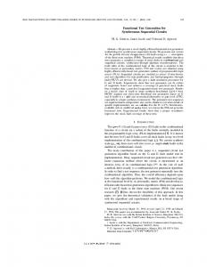
Fig. 1. A constructive cyclic circuit
electrically. An example taken from [7] (presented in Figure 1) consists of a cyclic circuit with two combinational subcircuits F and G. The circuit either computes y = G(F (x)) or y = F (G(x)), depending on the selection signal s. The circuit uses only one copy of F and G each and therefore contains a combinational cycle. However, the cycle is false in the sense that the output y is always well-defined. For a given cyclic circuit, a separate analysis of the circuit is needed to prove that all present cycles are false, or, in the terminology of [10], that the circuit is constructive. In 1994, Malik presented such an analysis for combinational circuits [7], which was extended by Shiple et al. to be able to deal with sequential circuits [10]. Their analysis produces a new circuit, which is functionally equivalent to the original circuit, but does not contain any cycles. This new circuit can then be analyzed by other formal verification tools in order to check formal properties of the circuit. The mentioned analyses are both based on BDDs [3]. This has as a drawback that circuits which are difficult to represent using BDDs are difficult to handle using the method, since the method inherently relies on computing a BDD which represents the function that the circuit implements. Also, the analyses involve a fixed point computation over BDDs, which might introduce extra costs. In 1999, Namjoshi et al. presented a circuit analysis method that does not require a fixed point iteration [8]. However, their method only works for combinational circuits, and to make the method usable for sequential circuits they resort to similar methods as the ones in [10]; decision diagrams are used to calculate the reachable states in the system. The main contribution of this paper is the following. We present a sound and complete automatic analysis method for circuits containing combinational loops that does not involve a fixed point iteration, calculating reachable states, or computing a new cycle-free circuit, that proves constructiveness of circuits. We use the basic idea from [8], but we use a propositional theorem prover 2
Claessen
(sometimes called SAT-solver) instead of decision diagrams. Then, we use temporal induction [9] to extend the method to sequential circuits. As said, the method does not compute a non-cyclic equivalent circuit. Instead, one can use the method directly to also prove possible safety properties of the circuit. The rest of the paper is organized as follows. The first three sections can be seen as a tutorial on the subject and introduce background material, large parts of which are also presented elsewhere; in Section 2, we introduce the definition of circuits, and what their naive, classical semantics is; in Section 3, we show how to verify safety properties of these circuits, under the classical semantics, using a propositional theorem prover; in Section 4, we present the constructive semantics of circuits, which corresponds more closely to what happens in electrical circuits. Our main result is presented in Section 5, where we show how safety properties of cyclic circuits can be proved, under the constructive semantics. Finally, in Section 6 we discuss related work and conclude.
2
Classical Semantics of Circuits
In this section, we introduce the model of combinational and sequential circuits we use in the paper, and what their classical semantics is. We closely follow the terminology from [1]. Combinational Circuits. A boolean formula is built up from variables, x, y, z, and operators 0, 1 (nullary), ¬ (unary), and ∧, ∨, ⇒, ⊕ (binary). A definition is written x = f , and consists of a boolean variable x and a formula f . A combinational circuit is a finite set C of definitions, such that, for every variable x, there is at most one definition of the form x = f in C. The restriction on multiple definitions is added because we do not want to talk about circuits which contain points which are driven by multiple signals. A variable x of a circuit C is called an input, if there is no definition of the form x = f contained in C. A solution of a combinational circuit is a valuation, i.e. an assignment of all variables to a boolean value 0 or 1, such that all definitions are satisfied, using the usual interpretation of the boolean operators. Sequential Circuits. A delayed definition is written x := y, and consists of two variables x and y. A sequential circuit (C, D) is a pair of a combinational circuit C and a finite set of delayed definitions D. Again, we apply the restriction that, for every variable x, there can be at most one definition of the form x = f in C or a delayed definition of the form x := y in D. A variable x is called an input of (C, D), if there is no definition in C of the form x = f and no delayed definition in D of the form x := y. 3
Claessen
In order to help defining the semantics of sequential circuits, we define the following renaming operations. Let i ≥ 1 be a natural number. For a combinational circuit C, we write C[i] for the copy of C, with each variable x replaced by a fresh variable xi . For a set of delayed definitions D, we write D[i] for the combinational circuit {xi = yi−1 | x := y ∈ D}. The initial state of the circuit is dealt with by defining D0 as the combinational circuit {y0 = 0 | x := y ∈ D}. Lastly, for a valuation s over variables x, we write s[i] for the valuation over labelled variables xi , for which it holds that s[i](xi ) = s(x). For a given sequential circuit (C, D), we define the combinational expansion, written (C, D)[k], as the combinational circuit: k [
C[i] ∪ D[i]
i=1
A sequence of valuations (s1 , . . . , sk ) is called a solution path of a sequential circuit (C, D), if (s1 [1] ∪ s2 [2] ∪ · · · ∪ sk [k]) is a solution of the combinational circuit D0 ∪ (C, D)[k].
3
Proving Safety Properties
In this section, we show how to automatically prove safety properties of combinational and sequential circuits. Safety Properties. For the purposes of this paper, a safety property is a particular variable p in the circuit that is supposed to be always true for all possible scenarios of a circuit. We say that, for a given combinational circuit C, a safety property p is valid, if s(p) = 1, for all solutions s of C. If we want the safety property to be a more complicated property than just a variable, namely a formula f , we can simply add p = f as a definition to C. In the rest of the paper, we will sometimes do this implicitly. For a sequential circuit (C, D), we say that a safety property p is valid, if, for all k, for all solution paths (s1 , . . . , sk ) of (C, D), and for all 1 ≤ i ≤ k, it is the case that si (p) = 1. Proving Combinational Properties. In order to check if a given property p is valid for a given combinational circuit C, we can use a propositional logic theorem prover, often called SAT-solver. There are many such theorem provers available. Our choice of theorem prover is discussed in Section 6. To check the validity of a safety property p, we simply prove: ^
x=f
x=f ∈C
4
!
⇒ p
Claessen
As is well-known, proving the validity of combinational safety properties is a co-NP-complete problem. Therefore, there are only worst-case exponential time algorithms known that can do this. Proving Sequential Properties. Next, we show how to check if a safety property p is valid for a given sequential circuit (C, D). Here, we use the method of temporal induction, as described in [9]. The idea is to prove the property in two steps: the base case, and the induction step. In the base case, we prove that the property holds in the initial state. This corresponds to proving that p is a valid property of the combinational circuit D0 ∪ (C, D)[1]. We can use the above method to do that. In the step case, we prove that if the property holds in a certain state, it will also hold in the next state. This corresponds to proving that p1 ⇒ p2 is valid in the combinational circuit (C, D)[2]. This can also be done with the method described above. Complete Induction. The method of temporal induction as described above is sound, but not complete. This means that there are safety properties which are valid but cannot be proved by the proposed method. In particular, when the safety property p is very weak, assuming it as an induction hypothesis is not enough for the induction step to be a valid formula. In order to make temporal induction complete, we add the notion of induction depth, which is a natural number d. We modify the base case such that it proves the property for the first d time steps, so that we can assume that the property holds for d steps in the induction step. Thus, the new base case is proving p1 ∧ · · ·∧ pd valid for the circuit D0 ∪ (C, D)[d]. The step case becomes proving p1 ∧ · · · ∧ pd ⇒ pd+1 valid for the circuit (C, D)[d + 1]. If a certain property is valid for the base case, but not the step case, we simply increase the induction depth d and try again. If the base case does not hold, we get a trace exhibiting the error back from the theorem prover. However, it is possible that this process never terminates. This can happen when the unreachable state space contains loops. To exclude the loops and to make the method complete, we can add an extra assumption in the step case, namely that all states used in it are unique. It is sound to assume this, since if there is a solution path leading to a state where p is not true, there also exists a solution path leading to that state which consists of unique states. So, we define Diff(D, i, j) to mean that the states in time instances i and j are different: ! ^ Diff(D, i, j) = ¬ xi = xj . x:=y∈D
5
Claessen
x=x∧x
x = ¬x
x = x ∨ ¬x
x= 0∧x
(a)
(b)
(c)
(d)
Fig. 2. Four cyclic circuits
The new induction step then amounts to proving the following formula valid for the circuit (C, D)[d + 1]: ! ^ Diff(D, i, j) ∧ p1 ∧ · · · ∧ pd ⇒ pd+1 . 1≤i