model is proposed for the wind vector, assuming that appropriate prior distributions for the ... distribution is too complicated to compute closed form expressions for the MAP and ... M (Ï,κ) denotes a VM distribution with mean direction Ï and concentration ..... [12] K. V. Mardia and P. E. Jupp, Directional statistics. Chichester,.
MCMC SAMPLING FOR JOINT SEGMENTATION OF WIND SPEED AND DIRECTION Nicolas Dobigeon and Jean-Yves Tourneret University of Toulouse, IRIT/INP-ENSEEIHT, BP 7122, 31071 Toulouse cedex 7, FRANCE {nicolas.dobigeon, jean-yves.tourneret}@enseeiht.fr
ABSTRACT The problem of detecting changes in wind speed and direction is considered. Bayesian priors, with various degrees of certainty, are used to represent relationships between the two time series. Segmentation is then conducted using a hierarchical Bayesian model that accounts for correlations between the wind speed and direction. A Gibbs sampling strategy overcomes the computational complexity of the hierarchical model and is used to estimate the unknown parameters and hyperparameters. The performance of the proposed algorithm is illustrated with results obtained with synthetic data. Index Terms— Monte Carlo methods, Bayesian inference, hierarchical model, joint segmentation, wind data. 1. INTRODUCTION Segmentation has received considerable attention in the literature (see for instance [1] and references therein). Off-line segmentation algorithms assume a collection of observations is available. One or multiple change-points instants are estimated from this collection. The change instants are estimated retrospectively (or equivalently detected retrospectively). This procedure explains the terminology “off-line” or “retrospective” used in the literature (see for instance [2]). The most common off-line segmentation strategies are based on the least squares principle [3], the maximum likelihood method or Bayesian strategies [4]. A common idea to all these strategies optimizes a criterion that depends upon the observed data, penalized by an appropriate cost function for preventing over-segmentation. The choice of the appropriate penalty for signal segmentation remains a fundamental problem. The penalty can be selected using the ideas of [3] in the framework of Gaussian model selection. However, this approach is difficult in practical applications where the noise level is unknown. Another idea views the penalty as prior information about the change-point locations within the Bayesian paradigm [5]. The segmentation is then conducted using the posterior distribution of the change locations. The choice of the prior distribution is of course very important since the segmentation performance strongly depends on this choice. Markov chain Monte Carlo (MCMC) methods are often considered when the posterior distribution is too complicated to be used to derive the Bayesian estimators of the change parameters, such as the maximum a posteriori (MAP) estimator or minimum mean square error (MMSE) estimator. It is important to mention here that Bayesian methods (possibly combined with MCMCs) have useful properties for signal segmentation. In particular, they allow estimation of the unknown model hyperparameters using hierarchical Bayesian algorithms [6, 7]. This paper studies the problem of jointly segmenting the wind speed and direction, recently introduced in [8]. A hierarchical Bayesian model is proposed for the wind vector, assuming that appropriate prior distributions for the unknown parameters are available. Vague
priors are assigned to the corresponding hyperparameters, that are then integrated out from the joint posterior distribution. An interesting property of the proposed approach is that it allows the estimation of the unknown model hyperparameters from the data (the hyperparameters could also be estimated by coupling MCMCs with an expectation-maximization algorithm as in [9]). Note that the proposed hierarchical algorithm differs from the algorithms developed in [8]. There the hyperparameters were fixed (by assuming the true value of the average of detected change is known) or adjusted from prior information regarding the tide hours. The hierarchical model developed in this paper estimates jointly the unknown parameters and hyperparameters from the observed data. There is a price to pay with the proposed hierarchical model. The change-point posterior distribution is too complicated to compute closed form expressions for the MAP and MMSE change-point estimators. This problem is solved by an appropriate Gibbs sampling strategy. The strategy draws samples according to the posteriors of interest and computes the Bayesian change-point estimators by using these samples. 1.1. Notation and problem formulation Determination of the statistical properties of the wind vector amplitude has been previously considered in the literature. The Weibull and lognormal distributions have been reported as the best distributions for wind speeds [10]. Choice of one of these depends upon many factors, including site location or low/strong wind intensities. The choice of these distributions is supported by many experiments with real data sets. This paper concentrates on the lognormal distribution. However, a similar analysis could be conducted for the Weibull distribution or the Rayleigh distribution (see [11] for more details). For the lognormal assumption, the statistical properties of the wind speed on the kth segment can be defined as follows: � y1,i ∼ LN mk , σk2 , (1) where k = 1, ..., K1 , i ∈ I1,k = {l1,k−1 + 1, ..., l1,k }, and the following notations have been used: � • LN m, σ 2 denotes a lognormal distribution with scale m and shape σ 2 , • K1 is the number of segments in the speed sequence y1 = [y1,1 , . . . , y1,n ] (n is the sample length). The wind direction is a circular random variable, described by a Von Mises (VM) distribution whose mean direction parameter varies from one segment to another: y2,i ∼ M (ψk , κ) ,
(2)
where k = 1, ..., K2 , i ∈ I2,k = {l2,k−1 + 1, ..., l2,k }, and the following notations have been used:
• M (ψ, κ) denotes a VM distribution with mean direction ψ and concentration parameters κ [12, p. 36], • K2 is the number of segments in the direction sequence y2 = [y2,1 , . . . , y2,n ]. For both the wind speed and direction sequences, the segment #k in the signal #j (j ∈ {1, 2}) has boundaries denoted by [lj,k−1 + 1, lj,k ], lj,k is the time index immediately after which a change occurs with the convention that lj,0 = 0 and lj,Kj = n. Finally, the wind speed y1 and direction y2 are assumed to be independent sequences. 1.2. Paper organization
2.1. Likelihoods The likelihood function of the wind speed sequence y1 can be expressed as follows: f (y1 |θ 1 ) ∝
K1 Y
2
σk2
�− n1,k 2
2
T −2mk S1,k +n1,k mk − 1,k 2 2σ
,
(3)
where θ 1 = (r1 , σ 2 , m), ∝ means “proportional to”, X X 2 T1,k = log2 (y1,i ) , S1,k = log (y1,i ) ,
(4)
e
k
k=1
i∈I1,k
i∈I1,k
This paper proposes a Bayesian framework and an efficient algorithm for estimating the change-point locations lj,k from the two observed time series yj , j ∈ {1, 2}. The Bayesian model requires appropriate priors for the change-point locations, wind speed and direction parameters. The Bayesian model also needs to adjust the corresponding hyperparameters. The proposed methodology assigns vague priors to the unknown hyperparameters. The priors are then integrated out from the joint posterior or estimated from the observed data. This results in a hierarchical Bayesian model described in Section 2. A Gibbs sampling strategy is studied in Section 3 and allows the generation of samples distributed according to the posterior of interest. Some simulation results for synthetic wind data are presented in Section 4. Conclusions are reported in Section 5.
and n1,k (r1 ) = l1,k − l1,k−1 denotes the length of segment #k in the wind speed sequence y1 . The likelihood function of the wind direction sequence y2 is:
2. HIERARCHICAL BAYESIAN MODEL
f (Y|θ) = f (y1 |θ 1 ) f (y2 |θ 2 ) ,
The joint segmentation problem is based upon estimation of the following unknown parameters
where the two densities appearing in the right hand side have been defined in (3) and (5).
• (K1 , K2 ) (numbers of segments), � • lj = lj,1 , . . . , lj,Kj for j ∈ {1, 2} (change-point locations), �T � • m = m1 , . . . , mK1 (wind speed scale parameters), �T � 2 (wind speed shape parameters), • σ 2 = σ12 , . . . , σK 1 �T � • ψ = ψ1 , . . . , ψK2 (wind direction means), • κ (wind direction concentration parameter). A standard re-parameterization [5, 7] introduces indicator variables rj,i (j ∈ {1, 2}, i ∈ {1, . . . , n}) such that: � rj,i = 1 if there is a change-point at time i in signal #j, rj,i = 0 otherwise, with rj,n = 1. This last condition ensures that the number of change-points and segments are equal for each signal, i.e. Pn Kj = the unknown i=1 rj,i . Using these indicator variables, � parameter vector is θ = {θ 1 , θ 2 }, where θ 1 = r1 , m, σ 2 , � � θ 2 = {r2 , ψ, κ} and rj = rj,1 , . . . , rj,n . Note that the parameter vector θ belongs to a space whose dimension depends on K1 and �K K2 , i.e., θ ∈ Θ = Θ1 × Θ2 with Θ1 = {0, 1}n × R × R+ 1 and Θ2 = {0, 1}n × [−π, π]K2 × R. This paper proposes a Bayesian approach for estimating the unknown parameter vector θ. Bayesian inference on θ is based on the �T � posterior distribution f (θ|Y), with Y = y1 , y2 , where f (θ|Y) is related to the observation likelihoods and the parameter priors via Bayes rule f (θ|Y) ∝ f (Y|θ)f (θ). The likelihood and priors are presented below for the joint segmentation of wind speed and direction.
K2 Y
f (y2 |θ 2 ) ∝
−κ
[I0 (κ)]−n2,k e
P
i∈I2,k
cos(y2,i −ψk )
,
(5)
k=1
where θ 2 = (r2 , ψ, κ), Ip (·) is the modified Bessel function of the first kind and order p and n2,k (r2 ) = l2,k − l2,k−1 denotes the length of segment #k in the wind direction sequence y2 . By assuming independence between the wind speed and direction sequences, conditioned on the change-point locations, the full likelihood function is: (6)
2.2. Parameter Priors 2.2.1. Indicators Correlations in the observed wind speed and direction signals are modeled by an appropriate prior distribution f (R|P), where � �T R = r1 , r2 and P is an hyperparameter defined below. A global abrupt change configuration is defined as a specific value of the matrix R composed of 0’s and 1’s, corresponding to a specific solution of the joint segmentation problem. Conversely, a local abrupt change configuration, denoted � ∈ E = {0, 1}2 , is a particular value of a column of R which corresponds to the presence/absence of changes at a given time in the two signals. Denote as P� the probability of having a local change configuration � at time i. First assume that P� does not depend on the time index i and � �T � �T that r1,i , r2,i is independent of r1,i0 , r2,i0 for any i 6= i0 . As a consequence, the indicator prior distribution expresses as: Y S (R) S00 S10 S01 S11 f (R|P) = P� � = P00 P10 P01 P11 , (7) �∈E
h
i where P� = Pr [r1,i , r2,i ]T = � , P = {P00 , P01 , P10 , P11 } = � �T {P� }�∈E and S� (R) is the number of times i such that r1,i , r2,i = �. Some comments regarding the prior distribution f (R|P) are appropriate. A value of P� near one indicates a very likely configu� �T ration r1,i , r2,i = � for all i = 1, . . . , n. For instance, choosing P00 ≈ 1 (resp. P11 ≈ 1) favors a simultaneous absence (resp. presence) of changes in the two observed signals. This choice introduces correlation between the change-point locations.
2.3.2. Hyperparameters γ and δ02
2.2.2. Wind speed parameter priors Inverse-Gamma distributions are elected as shape parameter priors: σk2 | ν, γ ∼ IG
�ν γ � , , 2 2
(8)
where IG(a, b) denotes the Inverse-Gamma distribution with parameters a and b, ν = 2 (as in [4]) and γ is an adjustable hyperparameter. This is the conjugate prior for the wind speed variance which has been used successfully in [4] for Bayesian curve fitting. Conjugate zero-mean Gaussian priors are chosen for the scale parameters: � mk | σk2 , δ02 ∼ N m0 , σk2 δ02 , (9) where m0 = 0 and δ02 is an adjustable hyperparameter. The conjugate priors allow one to easily integrate out the shape and scale parameters in the posterior f (θ|Y).
The priors for hyperparameters γ and δ02 are selected as a noninformative Jeffreys’ prior and a vague conjugate Inverse-Gamma distribution (i.e, with large variance). This choice reflects lack of precise knowledge of these hyperparameters: f (γ) =
1 1 + (γ), γ R
δ02 | ξ, β ∼ IG (ξ, β) .
(12)
Assume that the individual hyperparameters are independent. The full hyperparameter Φ prior distribution can then be written (up to a normalizing constant): ! Y α −1 1 � f (Φ | α, ξ, β) ∝ P� 1P (P) 1R+ (γ) γ �∈E (13) � � βξ β 2� × exp − 2 1R+ δ0 , Γ(ξ)(δ02 )ξ+1 δ0 R ∞ x−1 −t where Γ(x) = 0 t e dt is the Gamma function.
2.2.3. Wind direction parameter priors 2.4. Posterior distribution of θ Bayesian inference for VM distributions has been studied in [13], where appropriate priors for the VM parameters were defined. This paper uses the same prior, i.e, a conjugate VM distributions for wind mean directions: ψk | ψ0 , R0 , κ ∼ M (ψ0 , κR0 ) ,
The posterior distribution of the unknown parameter vector θ can be computed from the following hierarchical structure: Z Z f (θ|Y) = f (θ, Φ|Y)dΦ ∝ f (Y|θ)f (θ|Φ)f (Φ)dΦ,
(10)
(14) where
where R0 and ψ0 are fixed hyperparameters and a Jeffreys’ prior for the concentration parameter κ: f (κ) ∝
1 1 + (κ), κ R
f (θ|Φ) = f (R|P)
"K 1 Y
# f
� σk2 |ν, γ f
� mk |σk2 , δ02
k=1
(11)
where 1R+ (·) is the indicator function on R+ . This prior describes vague knowledge regarding the VM concentration parameter κ.
2.3. Hyperpriors The hyperparameter vector defined� above and associated with the parameter priors is Φ = P, γ, δ02 . Of course, the performance of the Bayesian segmenter for detecting changes in the two signals y1 and y2 depends strongly on these hyperparameter values. The proposed hierarchical Bayesian model allows estimation of these hyperparameters from the observed data. The hierarchical Bayesian model requires definition of the hyperparameter priors (hyperpriors). Summarized below are the hyperpriors for the joint segmentation of wind speed and direction.
×
The prior distribution for the hyperparameter P is a Dirichlet dis� �T tribution with parameter vector Pα = α00 , α01 , α10 , α11 defined on the simplex P = {P | �∈E P� = 1, P� ≥ 0} denoted as P ∼ D4 (α). This distribution is a classical prior for positive parameters summing to one. It allows marginalization of the posterior distribution f (θ|Y) with respect to P. Moreover, by choosing α� = α, ∀� ∈ E, the Dirichlet distribution reduces to the uniform distribution on P.
(15)
# f (ψk |κ, R0 , ψ0 ) f (κ) ,
k=1
and f (Y|θ) and f (Φ) are defined in (6) and (13). This hierarchical structure allows one to integrate out the nuisance parameters m, σ 2 , ψ and P from the joint distribution f (θ, Φ|Y), yielding: � � 1 f R, γ, δ02 , κ|Y ∝ 1R+ (κ) f δ02 |ξ, β C (R|Y, α) κ " � ν #K1 � �N Y � K2 � γ 2 I0 (Rk κ) 1 2 � × I0 (κ) I0 (R0 κ) Γ ν2 k=1 " # � �1 � K1 Y 2 1 ν + n1,k � 1 Γ × 2 1 + n1,k δ02 2
(16)
k=1
×
K1 Y k=1
2.3.1. Hyperparameter P
"K 2 Y
with
"
m20 − µ21,k 1 + δ02 n1,k 2 γ + T1,k + δ02
� #− n1,k 2
m0 + δ02 S1,k µ1,k = , 1 + δ02 n1,k 2 X 2 Rk = R0 cos ψ0 + cos y2,i i∈I2,k 2 X + R0 sin ψ0 + sin y2,i , i∈I2,k
,
(17)
and
and K1
Q
Γ (S� (R) + α� ) �. C (R|Y, α) = �P Γ �∈{0,1}2 (S� (R) + α� )
γ|R, σ 2 ∼ G
�∈{0,1}2
(18)
The posterior distribution in (16) is too complex to derive closedform expressions for the MAP or MMSE estimators for the unknown parameters. In this case, MCMC methods are implemented to generate samples that are asymptotically distributed according to the posteriors of interest. The samples can then be used to estimate the unknown parameters by replacing integrals with empirical averages over the MCMC samples. 3. A GIBBS SAMPLER FOR JOINT SIGNAL SEGMENTATION Gibbs sampling is an iterative sampling strategy. It consists of generating random samples (denoted by e·(t) where t is the iteration index) distributed according to the conditional posterior distributions of each parameter. This paper samples the distribution f (R, γ, δ02 , κ|Y) defined in (16) using the three step procedure outlined below. The main steps of the algorithm and the key equations are detailed in subsections 3.1 to 3.4. 3.1. Generation of samples according to f (R|γ, δ02 , κ, Y)
Let R−i denote the matrix R whose ith column has been removed. Thus h� i �T Pr r1,i , r2,i = �|R−i , γ, δ02 , Y ∝ f (Ri (�), γ, δ02 |Y), (19) where Ri (�) is the matrix R whose ith column has been replaced by the vector �. Equation in (19) yields a closed-form h� i expression of the �T probabilities Pr r1,i , r2,i = �|R−i , γ, δ02 , Y after appropriate normalization. � 3.2. Generation of samples according to f γ, δ02 |R, Y � To obtain samples distributed according to f γ, δ02 |R, Y , it is very convenient to generate vectors distributed according to the joint dis� tribution f γ, δ02 , σ 2 , m|R, Y by using Gibbs moves. Using the joint distribution (16), this step can be decomposed as follows: � • Generate samples according to f γ, σ 2 |R, δ02 , Y Integrating the joint distribution f (θ, Φ|Y) with respect to the scale parameters mk , the following results are obtained: ∼ IG (uk , vk ) ,
k = 1, . . . , K1
with ν + n1,k uk = 2 � 2 m20 − µ21,k 1 + δ02 n1,k γ + T1,k vk = + , 2 2δ02
(20)
,
(22)
where G(a, b) is the Gamma distribution with parameters (a, b). • Generate samples according to f (δ02 , m|R, σ 2 , Y) This is achieved as follows: � � m0 + δ02 S1,k δ02 σk2 2 2 mk |R, σ , δ0 , Y ∼ N , , 1 + δ02 n1,k 1 + δ02 n1,k (23) ! K1 X (mk − m0 )2 K1 2 2 ,β + δ0 |R, m, σ ∼ IG ξ + . 2 2σk2 k=1 (24) 3.3. Generation of samples according to f (κ|R, Y) To obtain samples distributed according to f (κ|R, Y), it is convenient to generate vectors distributed according to the joint distribution f (ψ, κ|R, Y) with Gibbs moves. This step can be done using the joint distribution f (θ, Φ|Y) and the following procedure: • Generate samples according to f (ψ|R, κ, Y) This is done as follows: k = 1, . . . , K2
where λk is the resultant length on the segment #k: P ! R0 sin ψ0 + i∈I2,k sin y2,i P λk = arctan , R0 cos ψ0 + i∈I2,k cos y2,i
(25)
(26)
and Rk is the corresponding direction given in (17). • Generate samples according to f (κ|R, ψ, Y) The conditional posterior distribution of κ is: � �N 1 1 f (κ|R, ψ, Y) ∝ 1R+ (κ) κ I0 (κ) � K2 � Y 1 × eκRk cos(ψk −λk ) . 2πI0 (R0 κ) k=1
(27) Therefore, samples can be taken from f (κ|R, ψ, Y) (by a simple Metropolis-Hastings procedure). The proposed distribution is a Gamma distribution κ? ∼ G (a, b). This choice is motivated ([12, p. 40]) by the asymptotic behavior of the modified Bessel function of order 0 (i.e. 1 I0 (x) ≈ (2πx)− 2 ex when x → ∞). The parameters a and b are chosen such that the mean of κ? is the maximum likelihood estimate κ bML and βκ2 is an arbitrary variance: a=
κ b2ML , βκ2
b=
κ bML . βκ2
(28)
Using the likelihood function f (y2 |r2 , κ, ψ), κ bML satisfies: K2 I1 (b κML ) 1 X X = cos (y2,i − ψk ) . I0 (b κML ) N i∈I k=1
(21)
!
k=1
ψk |R, κ, Y ∼ M (λk , Rk ) ,
This step is achieved by using a Gibbs sampler to generate Monte � � Carlo samples distributed according to f [r1,i , r2,i ]T |γ, δ02 , κ, Y . This vector is a random vector of Booleans in E. Consequently, its distribution is fully characterized by the probabilities h i Pr [r1,i , r2,i ]T = �|γ, δ02 , Y , � ∈ E.
σk2 |R, γ, δ02 , Y
K1 ν X 1 , 2 2σk2
(29)
2,k
The acceptance probability of the new state κ? is: � � f (κ? |R, ψ, Y) ga,b (κ) ? ρκ→κ = min 1, . f (κ|R, ψ, Y) ga,b (κ? )
(30)
3.4. Posterior distribution of P� The hyperparameters P� , � ∈ E, provide information about the correlation between the change locations in the two time series. It is useful to estimate them from their posterior distribution for practical applications. Straightforward computations yield the following Dirichlet posterior distribution for P: P|R, Y ∼ D4 (S� (R) + α� ).
(31)
4. SEGMENTATION OF SYNTHETIC WIND DATA The simulations presented in this section have been obtained for 2 sequences with sample size n = 250. The change-point locations are l1 = (140) for the wind speed sequence and l2 = (60, 140) for the wind direction sequence. The parameters of the first sequence are m = [1.1, 0.6]T and σ 2 = [0.05, 0.1]T . The parameters of � �T the second sequence are ψ = − π2 , − π6 , π3 and κ = 2. The fixed parameters and hyperparameters have been chosen as follows: ν = 2 (as in [4]), R0 = 10−2 and ψ0 = 0 (vague prior), ξ = 1 and β = 100 (vague hyperprior), α� = α = 1, ∀� ∈ E. The hyperparameters α� are equal, ensuring the Dirichlet distribution reduces to a uniform distribution. Moreover, the common value to the hyperparameters α� has been set to α = 1 � n in order to reduce the influence of this parameter in the posterior (31). The total number of runs for each Markov chain is NMC = 6000, including Nbi = 1000 burnin iterations. Thus only the last 5000 Markov chain output samples are used for the estimations. These values of NMC and Nbi ensure convergence of the sampler as shown in [11]. 4.1. Posterior distributions of the change-point locations The first simulation compares joint segmentation and signal-bysignal segmentations. Figure 1 shows the posterior distributions of the change-point locations in the two time-series, obtained for 1D segmentation (top) and for joint segmentation (bottom). These results show that the Gibbs sampler (when applied to the second time-series) has not been able to detect the second change in the second sequence (top). Conversely, this change-point is detected much more precisely when using the joint segmentation procedure (bottom). This result can be explained as follows. The presence of a change in the first time series favors the detection of this change in the second time series. Other simulations are available in [11] and confirms this behavior.
Fig. 1. Posterior distributions of the change-point locations for 1D (top) and joint segmentations (bottom) obtained after Nbi = 1000 burn-in iterations and Nr = 5000 iterations of interest.
4.2. Wind parameter estimation The estimates of the wind parameters (speed scale and shape parameters, mean directions and concentration parameters) are useful in practical applications requiring signal reconstruction. This section studies the estimated posterior distributions for the parameters corresponding to the previous synthetic wind data. The posterior distributions of the parameters mk (k = 1, . . . , K1 ) (conditioned upon K1 = 2) are depicted in figures 21 . They are clearly in good agreement with the actual values of these parameters m = [1.1, 0.6]T . The posterior distributions of the mean directions ψk (k = 1, . . . , K2 ) (conditioned upon K2 = 3) and the concentration parameter κ are depicted in figures 3 and 4. These posteriors are also in good agreement with the actual values of the parameters. 1 Similar
results have been obtained for the parameters σk2 , see [11].
Fig. 2. Posterior distributions of the wind speed scale parameters mk (for k = 1, 2) conditioned on K1 = 2.
5. CONCLUSIONS This paper studied a Bayesian sampling algorithm for segmenting wind speed and direction. The statistical properties of the wind speed and direction were described by lognormal and VM distributions with piecewise constant parameters. Posterior distributions of the unknown parameters provided estimates of the unknown param-
IEEE Trans. Signal Processing, vol. 46, no. 5, pp. 1365–1373, May 1998. [6] N. Dobigeon, J.-Y. Tourneret, and J. D. Scargle, “Joint segmentation of multivariate astronomical time series: Bayesian sampling with a hierarchical model,” IEEE Trans. Signal Processing, vol. 55, no. 2, pp. 414–423, Feb. 2007.
Fig. 3. Posterior distributions of the wind mean directions parameters ψk (for k = 1, 2, 3) conditioned on K2 = 3.
[7] N. Dobigeon, J.-Y. Tourneret, and M. Davy, “Joint segmentation of piecewise constant autoregressive processes by using a hierarchical model and a Bayesian sampling approach,” IEEE Trans. Signal Processing, vol. 55, no. 4, pp. 1251–1263, April 2007. [8] S. Reboul and M. Benjelloun, “Joint segmentation of the wind speed and direction,” Signal Processing, vol. 86, no. 4, pp. 744–759, April 2006. [9] E. Kuhn and M. Lavielle, “Coupling a stochastic approximation version of EM with an MCMC procedure,” ESAIM Probability & Statistics, vol. 8, pp. 115–131, 2004. [10] F. Giraud and Z. M. Salameh, “Steady-state performance of a grid-connected rooftop hybrid wind-PhotoVoltaic power system with battery storage,” IEEE Trans. Energy Conversion, vol. 16, no. 1, pp. 1–7, March 2001.
Fig. 4. Posterior distribution of the wind concentration parameter κ.
eters and their uncertainties. The proposed algorithm can be easily extended to other statistical models. For instance, joint segmentation of wave amplitude and direction described by Rayleigh and VM distributions was discussed. Simulation results conducted on synthetic signals illustrated the performance of the proposed methodology. This hierarchical Bayesian algorithm can handle other possible relationships between the two observed times series. For example, one typically has information that the different time series are more or less similar. This kind of vague, but important knowledge, is naturally expressed in a Bayesian context by the prior distributions adopted for the models and their parameters. Another important point is that information about the parameter uncertainties can be naturally extracted from the sampling strategy. This is typical of MCMC methods which explore the relevant parameter space by generating samples distributed according to the interesting posteriors. These samples can then be used to obtain confidence intervals and variances for the estimates of the unknown parameters. 6. REFERENCES [1] M. Basseville and I. V. Nikiforov, Detection of Abrupt Changes: Theory and Application. Englewood Cliffs NJ: Prentice-Hall, 1993. [2] C. Inclan and G. C. Tiao, “Use of cumulative sums of squares for retrospective detection of changes of variance,” J. Am. Stat. Assoc., vol. 89, pp. 913–923, 1994. [3] L. Birg´e and P. Massart, “Gaussian model selection,” Jour. Eur. Math. Soc., vol. 3, pp. 203–268, 2001. [4] E. Punskaya, C. Andrieu, A. Doucet, and W. Fitzgerald, “Bayesian curve fitting using MCMC with applications to signal segmentation,” IEEE Trans. Signal Processing, vol. 50, no. 3, pp. 747–758, March 2002. [5] M. Lavielle, “Optimal segmentation of random processes,”
[11] N. Dobigeon and J.-Y. Tourneret, “Joint segmentation of wind speed and direction using a hierarchical model,” Computational Statistics & Data Analysis, vol. 51, no. 12, pp. 5603– 5621, Aug. 2007. [12] K. V. Mardia and P. E. Jupp, Directional statistics. Chichester, England: Wiley, 2000. [13] K. V. Mardia and S. El-Atoum, “Bayesian inference for the Von-Mises distribution,” Biometrika, vol. 63, no. 1, pp. 203– 206, April 1976.