SAR IMAGE SIMULATION WITH APPLICATION TO TARGET ...

Progress In Electromagnetics Research, Vol. 119, 35–57, 2011

SAR IMAGE SIMULATION WITH APPLICATION TO TARGET RECOGNITION Y.-L. Chang1 , C.-Y. Chiang2 , and K.-S. Chen3, * 1 Department

of Electrical Engineering, National Taipei University of Technology, Taipei, Taiwan 2 Department

of Computer Science and Information Engineering, National Central University, Jhongli, Taiwan 3 Center

for Space and Remote Sensing Research, National Central University, Jhongli, Taiwan

Abstract—This paper presents a novel synthetic aperture radar (SAR) image simulation approach to target recognition, which consists of two frameworks, referred to as the satellite SAR images simulation and the target recognition and identification. The images simulation makes use of the sensor and target geo-location relative to the Earth, movement of SAR sensor, SAR system parameters, radiometric and geometric characteristics of the target, and target radar cross section (RCS), orbital parameters estimation, SAR echo signal generation and image focusing to build SAR image database. A hybrid algorithm that combines the physical optics, physical diffraction theory, and shooting and bouncing rays was used to compute the RCS of complex radar targets. Such database is vital for aided target recognition and identification system Followed by reformulating the projection kernel in an optimization equation form, the target’s reflectivity field can be accurately estimated. Accordingly, the target’s features can be effectively enhanced and extracted, and the dominant scattering centers are well separated. Experimental results demonstrate that the simulated database developed in this paper is well suited for target recognition. Performance is extensively tested and evaluated from real images by Radarsat-2 and TerraSAR-X. Effectiveness and efficiency of the proposed method are further confirmed.

Received 15 June 2011, Accepted 5 July 2011, Scheduled 19 July 2011 * Corresponding author: Kun-Shan Chen ([email protected]).

36

Chang, Chiang, and Chen

1. INTRODUCTION SAR (synthetic aperture radar) image understanding and interpretation is essential for remote sensing of earth environment and target detection [1–8]. In the development of aided target recognition and identification system SAR image database with rich information content plays important role. It is well recognized that these image base volumes are enormous and it is impractical to acquire it solely by insitu measurements. Hence, SAR simulation is one potential alternative to alleviating the problem. However, it is highly desirable to develop a full blown SAR image simulation scheme with high verisimilitude including the sensor and target geo-location relative to the Earth, movement of SAR sensor, SAR system parameters, radiometric and geometric characteristics of the target, and environment clutter The simulation should at least include the computation of target radar cross section (RCS), orbital parameters estimation, SAR echo signal generation, image focusing, and so on. Such simulation scheme is also well suited for satellite SAR mission planning. As an application example of the simulated SAR images, the second part of this paper is to deal with target recognition. Before doing so, feature enhancement and extraction is presented. It is well known that good feature enhancement is essential for target identification and recognition of SAR images [9, 10]. Novel algorithm proposed for spotlight mode SAR involves the formation of a cost function containing non-quadratic regularization constraints [11, 12]. In stripmap mode, neither the radar antenna nor the target being mapped rotate, and the radar flight track is almost perpendicular to look direction with a small squint angle. By reformulating the projection kernel and using it in an optimization equation form, an optimal estimate of the target’s reflectivity field may be obtained [13]. As a result, the image fuzziness may be reduced and image fidelity was preserved. Thus, the target’s features were adequately enhanced, and dominant scatterers can be well separated. Finally, target recognition from various commercial aircrafts was demonstrated through simulated database and a neural classifier. The neural network is structured to allow its training by Kalman filtering technique [14–18]. Performance evaluation was done from simulated images various real images by Radarsat-2 and TerraSAR-X in stripmap mode. 2. SATELLITE SAR IMAGES SIMULATION Figure 1 illustrates a functional block diagram of a satellite SAR image simulation and a follow up target recognition. The simulation

Progress In Electromagnetics Research, Vol. 119, 2011

37

Figure 1. SAR Image simulation and target recognition flowcharts. processing flow is basically adopted from [7, 19, 20]. Generally, the inputs include satellite and radar parameters setting, target’s CAD model, and also the clutter model. The computation includes satellite orbit estimation, imaging geometry, target RCS, SAR echo and raw signal generation. A critical step of Doppler centroid and rate estimation for image focusing is also included. The most time consuming part is in echo and raw signal generation which will be illustrated in detail below. Then a refined range-Doppler method is applied to perform the SAR image focusing. The outputs include sets of images for a desired target for a range of radar looking angles and orientation angles. Once the image database is built and made available, feature extraction and enhancement is performed, followed by a target recognition stage that includes a neural classifier training, and neural weights storage for later operation stage.

38

Chang, Chiang, and Chen

2.1. SAR Signal Model A typical side-looking SAR observation geometry is referred to Fig. 2 where the slant range between SAR and target, R is a function of satellite moving time or slow time η or equivalently depends on squint angle away from the zero-Doppler plane which corresponds to the slant range R0 . In SAR processing, it is essential to project R onto R0 .

Figure 2. A typical stripmap SAR observation geometry [19]. A SAR transmits a linear frequency modulated (LFM) signal of the form: ¡ ¢ st (τ ) = wr (τ, Tp ) cos 2πfc τ + παr τ 2 (1) where αr is chirp rate, Tp is pulse duration, fc is carrier frequency, τ is the ADC sampling time or fast time, and wr (·) is a rectangular function: ¯ ¯ µ ¶ ( ¯ ¯ τ 1, ¯ Tτp ¯ ≤ 0.5 wr (τ, Tp ) = rect = (2) Tp 0, else The received signal or raw data is a delayed version of the transmitted signal (1) [19], µ ¶ µ ¶ 2R 2R sr (τ ) = A0 st τ − = A0 wr τ − , Tp wa (η) c c ( ) µ ¶ µ ¶ 2R 2R 2 cos 2πf0 τ − + παr τ − +ϕ (3) c c where R is distance from antenna to a point target being observed, A0 is slant range backscatter coefficient of the target, ϕ is the phase term,

Progress In Electromagnetics Research, Vol. 119, 2011

39

Figure 3. A typical antenna pattern along the azimuth direction and received signal. and wa (η) is the antenna pattern and is a function of slow time. A commonly used pattern is of the form ) (√ 3θ(η) wa (η) ∼ (4) = sinc2 2βaz where βaz is the azimuth beamwidth, θ(η) is angle measured from boresight in the slant range plane. Fig. 3 displays such antenna pattern (upper) and received echo (lower) along the azimuth direction. The echo strength is varied according to antenna gain and is changed with flight time η Note that in synthetic aperture concept, the target’s information is embedded in Doppler frequency and its rate. The received signal is coherently mixed down to the baseband. After demodulation, the received signal is given as [19] µ ¶ 2R(η) s0 (τ, η) = A0 wr τ − , Tp wa (η) c ( ) µ ¶ 4πfc R(η) 2R(η) 2 exp −j + jπαr τ − + ϕ00 (5) c c where ϕ00 is lumped sum of phase noise from atmosphere, satellite altitude error, terrain, etc. and is only of interest for interferometric SAR. Eq. (5) serves as fundamental signal model for the working process that follows. 2.2. RCS Computation To facilitate the radar response from a target, we need the target’s RCS under radar observation scenario. The radar backscattering

40

Chang, Chiang, and Chen

(a)

(b)

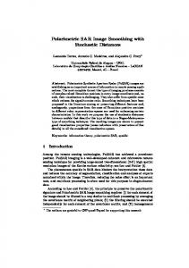
Figure 4. Computed RCS of commercial aircrafts for (a) C-band HH polarization, (b) X-band V V polarization. characteristics is taken into account. The coherent scattering process between target and its background is neglected for sake of simplicity. Also, fully polarimetric response is not considered. The Radar Cross Section Analysis and Visualization System (RAVIS) [21] is a powerful algorithm that utilizes the physical optics (PO), physical diffraction theory (PDT), and shooting and bouncing rays (SBR) to compute the RCS of complex radar targets [22, 23]. Single scattering and diffraction from a target are first computed by PO and PDT, followed by SBR to account for multiple scattering and diffraction. The system outputs for a given 3D CAD model of the target of interest The CAD model contains numerous grids or polygons, each associated with the computed RCS as a function of incident and aspect angles for a given set of radar parameters. The number of polygons is determined by target’s geometry complexity and its electromagnetic size. To realize the imaging scenario, each polygon must be properly oriented and positioned based on Earth Centered Rotating (ECR) coordinates. Fig. 4 displays the computed RCSs of these aircraft for the cases of Radarsat-2 and TerraSAR-X. 2.3. Clutter Model Although the coherent scattering process between target and its background is neglected for sake of simplicity, the clutter from

Progress In Electromagnetics Research, Vol. 119, 2011

41

background is incoherently integrated into the radar echo. Extensive studies on SAR speckle and its reduction have been documented [8, 24– 26]. Many studies [27, 28] suggest that for surface-like clutter such as vegetation canopy [29, 30] and airport runway, the radar signal statistics follows fairly well Weibull distribution. For our aircraft targets of interest, we applied the Weibull distribution for runway clutter model. Other models can be easily adopted in the simulation chain. κ ³ x ´κ−1 exp [−(x/λ)κ ] (6) p (x) = λ λ where the shape parameter κ and scale parameter λ may be estimated from real SAR images over the runway with mean amplitude A [26] π √ κ = (7) std [ln (A)] 6 ½ ¾ 0.5722 λ = exp [< ln (A) >] + (8) κ Fig. 5 displays sample regions of clutter and estimated model parameters on a TerraSAR-X image. The model parameters are obtained by averaging several samples.

Figure 5. Samples of clutter and estimated model parameters on a TerraSAR-X image.

42

Chang, Chiang, and Chen

2.4. Satellite Orbit Determination In applying Eq. (5), the range between a satellite in space and a target being imaged on the ground must be precisely determined for matched filtering. That is to say we need to know the satellite and target position vectors in order to estimate the Doppler frequency and its rate. Before doing so we have to define and then determine the reference systems for time. Also the transformation between geocentric and geodetic coordinates on the Earth must be computed. Six fundamental parameters required to determine the orbital position include semimajor axis a, eccentricity e, inclination angle i, right ascension of ascending node Ω, argument of perigee ω, true anomaly ν. Three of the parameters determine the orientation of the orbit or trajectory plane in space, while three locate the body in the orbital plane [31, 32]. These six parameters are uniquely related to the position and velocity of the satellite at a given epoch. To deduce the orbital elements of a satellite, at least six independent measurements are needed [31]. In this paper, we adopted simplified perturbations models (SPM) [33–35] to estimate the orbital state vectors of satellite in the Earth Centered Inertial (ECI) coordinate system. A C++ version program code by Henry [33] was used. Once the orbit parameters are determined, we can transform it to ECR coordinate system, as described below. The transformation matrix is of the form [31] UECI ECR = ΠΘNP

(9)

where matrices Π, Θ, N, P represent, respectively, polar motion, Earth rotation, nutation, and precession matrices: Θ (t) = Rz (GAST ) P (T1 , T2 ) = Rz (−z (T, t)) Ry (ϑ (T, t)) Rz (−ξ (T, t))

(10) (11)

where GAST is Greenwich apparent sidereal time. Referring to Fig. 6, the nutation matrix is N (T ) = Rx (−ε − ∆ε) Rz (−∆ψ) Rz (ε)

(12)

Note that from [31], in computing the derivative of the transformation, the precession, nutation and polar motion matrix maybe considered as constant. dUECI dΘ ECR ≈Π NP dt dt

(13)

Progress In Electromagnetics Research, Vol. 119, 2011

43

Figure 6. Illustration of nutation. Then the state vectors in the transformation are rECR = UECI ECR rECI

(14) dUECI ECR

vECR = UECI ECR vECI + dt ¡ ECI ¢T rECI = UECR rECR

rECI

¡ ¢T ¡ ECI ¢T d UECI ECR rECR vECI = UECR vECR + dt In summary, four key steps are needed:

(15) (16) (17)

(i) Find satellite position: calculated from two-line elements data and imaging time duration; (ii) Find radar beam pointing vector derived from satellite attitude (pitch, roll and yaw angle); (iii) Locate target center position derived from satellite position and line of sight; (iv) Locate each target’s polygon position derived from target center position and target aspect angle. 2.5. Image Focusing Several focusing algorithms have been proposed including RangeDoppler (RD), Omega-K, Chirp-Scaling, etc. [19, 36, 37] and their improved versions Each of them bears pros and cons. We adopted the refined range-Doppler algorithm with secondary range compression because of their fast computation while maintaining reasonable good spatial resolution and small defocusing error. Fig. 7 outlines the functional block diagram of processing steps in refined RD algorithm.

44

Chang, Chiang, and Chen START

Orbit Data

SAR Raw Data

Baseband Doppler Centroid Frequency Estimation (PB/ACCC)

Azimuth Matching Filter Generation

Doppler Frequency Ambigulity Estimation (WDA/MLCC/MLBF)

Azimuth Compression

Absolute Doppler Centroid Frequency

SAR Image

Range Compression

Good Enough

Range Migration Cells Correction (Sinc Insterpolation )

Autofocusing (Optional)

NO

YES

STOP Doppler Rate Estimation (Effective Velocity)

PB (Power Balance) ACCC (Average Cross Correlation Coefficient) MLCC (Multi-Look Cross-Correlation) MLBF (Multilook Beat Frequency) WDA (Wavenumber Domain Algorithm)

Figure 7. SAR image focusing flowchart of a RD-based algorithm. The power balance method in conjunction with the average cross correlation coefficient method was used to obtain a rough estimate of baseband Doppler frequency [38]. To obtain absolute Doppler centroid frequency, fDC , algorithms such as MLCC (Multi-Look Cross-Correlation), MLBF (Multilook Beat Frequency), and WDA (Wavenumber Domain Algorithm) may be utilized to determine the ambiguity number [19]: fDC = fDC,base + Mamb P RF

(18)

where fDC,base is the baseband part of PRF, Mamb is ambiguity number and PRF is pulse repetition frequency. After an effective satellite velocity, Vr , is estimated from orbit state vectors, the Doppler rate estimation can be computed via fR (R0 ) =

2Vr2 (R0 ) cos (θsq,c ) R0

(19)

Progress In Electromagnetics Research, Vol. 119, 2011

45

where θsq,c is squint angle, and R0 is referred to zero-Doppler plane (See Fig. 2). Note that in some cases, Eq. (19) is just a rough estimate. Then autofocus via phase gradient algorithm [19] may be further applied to refine the Doppler rate given above. 3. APPLICATION TO TARGET RECOGNITION The proposed working flows and algorithms were validated by evaluating the image quality including geometric and radiometric accuracy using simple point targets first, followed by simulating four types of commercial aircrafts: A321 B757-200, B747-400, and MD80 The satellite SAR systems for simulation include ERS-1, ERS-2, Radarsat-2, TerraSAR-X, and ALOS PALSAR, but others can be easily realized. Table 1 lists the key image quality indices for a simulated image of TerraSAR-X and PLASAR satellite SAR systems. Quality indices include 3 dB azimuth beamwidth (m), peak-to-side lobe ratio (dB), integrated side lobe ratio (dB), scene center accuracy in different coordinate systems. As can be seen from the table, the simulated images are all well within the nominal specifications for different satellite systems.

Table 1. Comparison of simulated image quality for a point target. ALOS PALSAR TerraSAR-X Simulation Nominal Simulation Nominal 3 dB Azimuth beamwidth [m] 4.26 3.49 5.10 4.51 − 24.85 Slant range −22.85 PSLR [dB] −20.5 −13 Azimuth − 25.42 −31.16 Slant range − 30.62 −31.62 ISLR [dB] −15.0 −17 Azimuth − 25.62 −43.98 o o o 121.49927 E, 121.49930 E, 119.395090 E, 119.39506oE, Lon, Lat [degree] 24.764622 oN 24.764477oN 24.894470oN 24.894620 oN −3027814.2, −3027808.4, −2817396.77, −2817397.45, ECR(x,y,z) [m] 4941079.3, 4941075.0, 5608995.60, 5608996.11, 2655407.1 2655421.7 2830631.97 2830630.29 Scente cener Lon/Lat difference -5 -4 -6 −3x10 , 1.45x10 −3x10 , 1.5x10-4 [degree] ECR difference (ground range, 0.98, −16.26 0.06, 16.97 azimuth) [m] Index

46

Chang, Chiang, and Chen

3.1. Feature Enhancement The essential information for target classification, detection, recognition, and identification is through feature selection for training phase. For our interest, depending on the spatial resolution offered by Radarsat-2 and TerraSAR-X in stripmap mode, we aim at target recognition. Before feature extraction, feature enhancement is performed first. To enhance the SAR data using the non-quadratic regularization method [11, 12], one has to modify the projection operator kernel accordingly. The received signal so in Eq. (5) may be expressed as [13]: so = Tf + sn (20) where sn represents noise, and T is the projection operation kernel with dimension M N × M N which plays a key role in contrast enhancement if the signal in Eq. (5) is of dimension M ×N . It has been shown that [1] non-quadratic regularization is practically effective in minimizing the clutter while emphasizing the target features via: n o ˆ f = arg min ksr − Tf k22 + γ 2 kf kpp (21) where kkp denotes `p -norm (p ≤ 1), and γ 2 is a scalar parameter and n o kso − Tf k22 + γ 2 kf kpp is recognized as the cost or objective function. To easily facilitate the numerical implementation, both so and f may be formed as long vectors, with T a matrix. Then, from Eq. (5) and Eq. (20), we may write the projection operation kernel for the stripmap mode as [13]   ³ ³ ´ ´ 2   (x−x0 )2 (x−x0 )2     2 r+ 2r  2 r+ 2r    (22) T = exp −iω0 −α t−    c c   where t, r, x − x0 are matrices to be described below by firstly defining the following notations to facilitate the formation of these matrices: N : the number of discrete sampling points along the slant range direction, M : the number of discrete sampling points along the azimuth direction, Dt: the sampling interval along the slant range, `r : the size of the footprint along the slant range, `x : the size of the footprint along the azimuth direction, 1l : the column vector of dimension l × 1 and all of elements equal to one, in which l = M or l = M N .

Progress In Electromagnetics Research, Vol. 119, 2011

47

With these notions, we can obtain explicit t, r, x − x0 forms, after some mathematical derivations [13]. t = [1M ⊗ M1 ]M N ×M N    0  1    ∆t =  v1 =  .  ..   N −1 M1 = V1 · 1TM N



(23)  0 ∆t   ..  . (N − 1)∆t N ×1

0 ···  ∆t =  ... (N − 1)∆t · · ·

r = [M2 ⊗ V2T ]M N ×M N  −` r 2 + r0  −`r + r0 + ∆`  V2 =  . 2  .. −`r 2

M2 =

1TM

⊗ 1M N

 0 ∆t   (24b) ..  . (N − 1)∆t N ×M N (25)

    

+ r0 + (N − 1)∆` = [ 1M N

(24a)

, ∆` =

`r N

(26a)

N ×1

· · · 1M N ]M N ×M N

x − x0 = [M3 ⊗ M4 ]M N ×M N

(26b) (27)

 −`   x 0 2 `x `x   1  `x `x   M − 2   − = V3 =  (28a)   . .  .. M 2  ..  `x M −1 (M − 1) M − `2x M ×1 ¸ ¹ º · M −1 V3 [δ − 1 : (M − 1)]δ×1 ; δ= +1 (28b) V4 = 0 2 (M −δ)×1 M ×1 · ¸ Mirror(V3 [0 : δ − 1])δ×1 V5 = 0 (28c) 

(M −δ)×1

M ×1

£ ¤ M3 = Toep(V5T , V4T ) M ×M (28d) £ ¤ T M4 = 1N ×1 · 1N ×1 N ×N (28e) In the above equations, each of the bold-faced letters denotes a matrix, and ⊗ represents the Kronecker product. The operation V[m : n] takes element m to element n from vector V, and Toep( · ) converts the input into a Toeplitz matrix [39, 40]. Note that in (28c),

48

Chang, Chiang, and Chen

by Mirror [a : b, c : d]p×q we mean taking elements a to b along the rows and elements c to d along the columns, so that the resulting matrix is of size p × q. 3.2. Feature Vectors and Extraction The feature vector contains two types: fractal geometry and scattering characteristics. In fractal domain, the image is converted into fractal image [41]. It has been explored that SAR signals may be treated as a spatial chaotic system because of the chaotic scattering phenomena [42, 43]. Applications of fractal geometry to the analysis of SAR are studied in [44, 45]. There are many techniques proposed to estimate the fractal dimension of an image. Among them, the wavelet approach proves both accurate and efficient. It stems from the fact that the fractal dimension of an N -dimensional random process can be characterized in terms of fractional Brownian motion (fBm) [41]. The power spectral density of fBm is written as P (f ) ∝ f −(2H+D)

(29)

where 0 < H < 1 is the persistence of fBm, and D is the topological dimension (= 2 in image). The fractal dimension of this random process is given by D = 3 − H. As image texture, a SAR fractal image is extracted from SAR imagery data based on local fractal dimension. Therefore, wavelet transform can be applied to estimate the local fractal dimension of a SAR image. From (29), the power spectrum of an image is therefore given by ³p ´−2H−2 P (u, v) = υ u2 + v 2 (30) where υ is a constant. Based on the multiresolution analysis, the discrete detailed signal of an image I at resolution level j can be written as [46, 47]: ¡ ¢® ­ Dj I = I (x, y) , 2−j Ψj x − 2−j n, y − 2−j m ¡ ¢¡ ¢ = I (x, y) ⊗ 2−j Ψj (−x, −y) 2−j n, 2−j m (31) ¡ ¢ where ⊗ denotes a convolution operator, Ψj (x, y) = 22j Ψ 2j x, 2j y and Ψ (x, y) is a two-dimensional wavelet function. The discrete detailed signal, thus, can be obtained by filtering the signal with 2−j Ψj (−x, −y) and sampling the output at a rate 2−j . The power spectrum of the filtered image is given by [47] ¯ ¯2 ¯˜ ¯ Pj (u, v) = 2−2j P (u, v) ¯Ψ (32) j (u, v)¯

Progress In Electromagnetics Research, Vol. 119, 2011

49

¡ ¢ ˜ j (u, v) = Ψ ˜ 2−j u, 2−j v and Ψ ˜ (u, v) is the Fourier transform where Ψ of Ψ (u, v). After sampling, the power spectrum of the discrete detailed signal becomes XX ¡ ¢ Pjd (u, v) = 2j Pj u + 2−j 2kπ, v + 2−j 2lπ (33) k

Let

σj2

l

be the energy of the discrete detailed signal ZZ 2−j 2 σj = Pjd (u, v) dudv (2π)2

(34)

By inserting (32) and (33) into (34) and changing variables in this 2 . Therefore, the integral, (34) may be expressed as σj2 = 2−2H−2 σj−1 fractal dimension of a SAR image can be obtained by computing the ratio of the energy of the detailed images: D=

σj2 1 log2 2 + 2 2 σj−1

(35)

A fractal image indeed represents information regarding spatial variation; hence, its dimension estimation can be realized by sliding a preset size window over the entire image. The selection of the window size is subject to reliability and homogeneity considerations with the center pixel of the window replaced by the local estimate of the fractal dimension. Once fractal image is generated, features of angle, target area, long axis, short axis, axis ratio are extracted from target of interest. As for scattering center (SC), features of major direction [X], major direction [Y ], minor direction [X], minor direction [Y ], major variance, and minor variance are selected, in addition to radar look angle and aspect angle. Fig. 8 displays such feature vector from simulated MD80 and B757-200 aircrafts from Radarsat-2. Finally, the recognition is done by a dynamic learning neural classifier [14–18]. This classifier is structured with a polynomial basis function model. A digital Kalman filtering scheme [48] is applied to train the network. The necessary time to complete training basically is not sensitive to the network size and is fast. Also, the network allows recursive training when new and update training data sets is available without revoking training from scratch. The classifier is structured with 13 input nodes to feed the target features, 350 hidden nodes in each of 4 hidden layers, and 4 output nodes representing 4 aircraft targets (A321, B757-200, B747-400, and MD80).

50

Chang, Chiang, and Chen

(a)

(b)

Figure 8. Selected features of simulated Radarsat-2 images of (a) A321 and (b) B757-200 for incidence angle of 35◦ and aspect angle from −180◦ ∼ +179 o (1◦ step).

3.3. Performance Evaluation 3.3.1. Simulated SAR Images Both simulated Radarsat-2 and TerraSAR-X images for 4 targets, as described above, are used to evaluate the classification and recognition performance. For this purpose, Radarsat-2 images with incidence angle of 45◦ and TerraSAR-X with 30◦ of incidence were tested. Both are with spatial resolution of 3 m in stripmap mode. The training data contains all 360 aspect angles (1◦ a step), among them 180 samples were randomly taken to test. Fast convergence of neural network learning is observed. The confusion matrix for Radarsat-2 and TerraSAR-X in classifying 4 targets is given in Table 2 and Table 3, respectively. The overall accuracy and kappa coefficient are very satisfactory. Higher confusion between B757-200 and MD80 was observed. It has to be noted that with Radarsat-2 and TerraSAR-X systems, comparable results were obtained as long as classification rate is concerned.

Progress In Electromagnetics Research, Vol. 119, 2011

51

Table 2. Confusion matrix of classifying 4 targets from simulated Radarsat-2 images. A321

B747-400 B757-200 MD80

A321 B747-400 target B757-200 MD80

165 0 4 4

2 175 1 2

6 3 164 11

7 2 11 163

User accuracy

0.954

0.972

0.891

0.891

Producer accuracy 0.917 0.972 0.911 0.906

overall accuracy: 0.926, kappa coefficient: 0.902

Table 3. Confusion matrix of classifying 4 targets from simulated TerraSAR-X images. A321

B747-400 B757-200 MD80

Producer accuracy

A321 B747-400 target B757-200 MD80

166 0 2 1

0 179 0 0

5 0 168 8

9 1 10 171

0.922 0.994 0.933 0.950

User accuracy

0.954

0.982

1.000

0.928

0.895

overall accuracy: 0.950, kappa coefficient: 0.933

3.3.2. Real SAR Images Data acquisition on May 8, 2008 from TerraSAR-X over an airfield was processed into 4 looks images with spatial resolution of 3 m in stripmap mode. Feature enhancement by an operator kernel in (22) was performed. Meanwhile, ground truth collections were conducted to identify the targets. Fig. 9 displays such acquired images where the visually identified targets are marked and their associated image chips were later fed into neural classifier that is trained by the simulated image database. Among all the targets, 3 types of them are contained in simulated database: MD80, B757-200, and A321. From Table 4, these targets are well recognized, where the numeric value represents membership. Winner takes all approach was taken to determine the classified target and whether they are recognizable. More sophisticated schemes such as type-II fuzzy may be adopted in the future. It is realized that for certain poses, there exists confusion between MD80 and B757-200, as already demonstrated in simulation test above. As another example, a blind test was performed. Here blind means

52

Chang, Chiang, and Chen

Table 4. Membership matrix for target recognition on TerraSAR-X image of Fig. 9. PP

PPoutput A321 B747-400 B757-200 MD80 recognizable PP input P MD80 1 16.61% 7.26% 0.00% 76.12% yes MD80 2

0.00%

9.63%

18.50%

71.85%

yes

MD80 3

0.00%

3.63%

8.78%

87.58%

yes

MD80 4

0.00%

3.64%

23.08%

73.27%

yes

MD80 5

17.88%

12.28%

0.00%

69.82%

yes

MD80 6

5.64%

0.00%

46.72%

47.63%

yes

B757-200 1

12.05%

11.84%

76.09%

0.00%

yes

B757-200 2

0.00%

19.41%

78.55%

2.03%

yes

A321

63.28%

15.09%

0.00%

21.61%

yes

Figure 9. A TerraSAR-X image over an airfield acquired on May 15, 2008. The identified targets are marked from ground truth. the targets to be recognized is not known to the tester, nor is the image acquisition time. The ground truth was collected by the third party and was only provided after recognition operation was completed. This is very close to the real situation for recognition operation. A total of 12 targets (T1-T12) were chosen for test, as indicated in Fig. 10. Unlike in Fig. 9, this image was acquired in descending mode but was unknown at the time of test. Table 5 gives the test results, where the recognized targets and truth are listed. It is readily indicated that all the MD80 targets were successfully recognized, while 4 types of targets were wrongly recognized. T12 target (ground truth is a

Progress In Electromagnetics Research, Vol. 119, 2011

53

Figure 10. A Radarsat-2 image over an airfield. The identified targets are marked. Table 5. Membership matrix for target recognition on Raradsat-2 image of Fig. 10. HH

HH A321 H

T1

B747-400 B757-200 MD80 Recognized

19.25%

0.00%

T2

0.01%

T3

14.99%

T4

Truth

22.88%

57.86%

MD80

MD80

0.00%

0.00%

99.98%

MD80

MD80

0.00%

11.59%

73.40%

MD80

MD80

21.31%

10.81%

15.27%

52.60%

MD80

MD80

T5

0.00%

3.09%

95.10%

1.79%

B757-200

E190

T6

96.82%

1.70%

0.00%

1.46%

A321

B737-800

T7

0.13%

0.00%

0.17%

99.69%

MD80

MD80

T8

0.10%

0.04%

0.00%

99.84%

MD80

MD80

T9

63.28%

15.09%

0.00%

21.61%

A321

FOKKER-100

T10

6.48%

2.26%

0.00%

91.24%

MD80

MD80

T11

43.61%

15.59%

40.59%

0.00%

A321

DASH-8

C130) was completely not recognizable by the system. These are mainly attributed the lack of database. Consequently enhancement and update of the target database is clearly essential. 4. CONCLUSION In this paper, we present a full blown satellite SAR image simulation approach to target recognition. The simulation chain includes orbit state vectors estimation, imaging scenario setting, target

54

Chang, Chiang, and Chen

RCS computation, clutter model, all specified by a SAR system specification. As an application example, target recognition has been successfully demonstrated using the simulated images database as training sets. Extended tests on both simulated image and real images were conducted to validate the proposed algorithm. To this end, it is suggested that a more powerful target recognition scheme should be explored for high-resolution SAR images. Extension to fully polarimetric SAR image simulation seems highly desirable as more such data are being available for much better target discrimination capability. In this aspect, further improvement on the computational efficiency by taking advantage of graphic processing unit (GPU) power may be preferred and is subject to further analysis. REFERENCES 1. Rihaczek, A. W. and S. J. Hershkowitz, Theory and Practice of Radar Target Identification, Artech House, 2000. 2. Huang, C. W. and K. C. Lee, “Frequency-diversity RCS based target recognition with ICA projection,” Journal of Electromagnetic Waves and Applications, Vol. 24, No. 17–18, 2547–2559, 2010. 3. Guo, K. Y., Q. Li, and X. Q. Sheng, “A precise recognition method of missile warhead and decoy in multi-target scene,” Journal of Electromagnetic Waves and Applications, Vol. 24, No. 5–6, 641– 652, 2010. 4. Tian, B., D. Y. Zhu, and Z. D. Zhu, “A novel moving target detection approach for dual-channel SAR system,” Progress In Electromagnetics Research, Vol. 115, 191–206, 2011. 5. Wang, X. F., J. F. Chen, Z. G. Shi, and K. S. Chen, “Fuzzycontrol-based particle filter for maneuvering target tracking,” Progress In Electromagnetics Research, Vol. 118, 1–15, 2011. 6. Lee, J. S. and E. Pottier, Polarimetric Radar Imaging: From Basics to Applications, CRC Press, 2009. 7. Margarit, G., J. J. Mallorqui, J. M. Rius, and J. Sanz-Marcos, “On the usage of GRECOSAR, an orbital polarimetric SAR simulator of complex targets, to vessel classification studies,” IEEE Trans. Geoscience and Remote Sens., Vol. 44, 3517–3526, 2006. 8. Lee, J. S., “Digital image enhancement and noise filtering by use of local statistics,” IEEE Trans. Pattern Anal. Mach. Intell., Vol. 2, 165–168, 1980. 9. Chang, Y. L., L. S. Liang, C. C. Han, J. P. Fang, W. Y. Liang, and K. S. Chen, “Multisource data fusion for landslide classification

Progress In Electromagnetics Research, Vol. 119, 2011

10.

11. 12.

13.

14. 15.

16.

17.

18. 19. 20.

55

using generalized positive boolean functions,” IEEE Trans. Geosci. Remote Sensing, Vol. 45, 1697–1708, 2007. Wang, J. and L. Sun, “Study on ship target detection and recognition in SAR imagery,” CISE’09 Proceedings of the 2009 First IEEE International Conference on Information Science and Engineering, 1456–1459, 2009. C ¸ etin, M. and W. C. Karl, “Feature-enhanced synthetic aperture radar image formation based on nonquadratic regularization,” IEEE Trans. on Image Processing, Vol. 10, 623–631, 2001. C ¸ etin, M., W. C. Karl, and A. S. Willsky, “Feature-preserving regularization method for complex-valued inverse problems with application to coherent imaging,” Optical Engineering, Vol. 45, 017003-1–11, 2006. Chiang, C. Y., K. S. Chen, C. T. Wang, and N. S. Chou, “Feature enhancement of stripmap-mode SAR images based on an optimization scheme,” IEEE Geoscience and Remote Sensing Letters, Vol. 6, 870–874, 2009. Tzeng, Y., K. S Chen, W. L. Kao, and A. K. Fung, “A dynamic learning neural network for remote sensing applications,” IEEE Trans. Geosci. Remote Sensing, Vol. 32, 1096–1102, 1994. Chen, K. S., Y. C. Tzeng, C. F. Chen, and W. L. Kao, “Land-cover classification of multispectral imagery using a dynamic learning neural network,” Photogrammet. Eng. Remote Sensing, Vol. 61, 403–408, 1995. Chen, K. S., Y. C. Tzeng, and W. L. Kao, “Retrieval of surface parameters using dynamic learning neural network,” International Geoscience and Remote Sensing Symposium 1993, IGARSS ’93. Better Understanding of Earth Environment, Vol. 2, 505–507, 1993. Chen, K. S., W. P. Huang, D. W. Tsay, and F. Amar, “Classification of multifrequency polarimetric SAR image using a dynamic learning neural network,” IEEE Trans. Geosci. Remote Sensing, Vol. 34, 814–820, 1996. Tzeng, Y. C. and K. S. Chen, “A fuzzy neural network to SAR image classification,” IEEE Trans. Geosci. Remote Sensing, Vol. 36, 301–307, 1998. Cumming, I. and F. Wong, Digital Signal Processing of Synthetic Aperture Radar Data: Algorithms and Implementation, Artech House, 2004. Curlander, J. C. and R. N. McDonough, Synthetic Aperture Radar: Systems and Signal Processing, Wiley-Interscience, 1991.

56

Chang, Chiang, and Chen

21. Chen, C. C., Y. Cheng, and M. Ouhyoung, “Radar cross section analysis and visualization system,” Proceeding of Computer Graphics Workshop 1995, 12–16, Taipei, Taiwan, 1995. 22. Lee, H., R. C. Chou, and S. W. Lee, “Shooting and bouncing rays: Calculating the RCS of an arbitrarily shaped cavity,” IEEE Trans. Antennas Propag., Vol. 37, 194–205, 1989. 23. Chen, S. H. and S. K. Jeng, “An SBR/image approach for indoor radio propagation in a corridor,” Trans. IEICE Electron., Vol. E78-C, No. 8, 1058–1062, 1995. 24. Lee, J. S., “Refined filtering of image noise using local statistics,” Comput., Vis., Graph., Image Process., Vol. 15, 380–389, 1981. 25. Lee, J. S., M. R. Grunes, and R. Kwok, “Classification of multi-look polarimetric SAR imagery based on complex Wishart distribution,” Int. J. Remote Sensing, Vol. 15, 2299–2311, 1994. 26. Lee, J. S., P. Dewaele, P. Wambacq, A. Oosterlinck, and I. Jurkevich, “Speckle filtering of synthetic aperture radar images: A review,” Remote Sens. Rev., Vol. 8, 313–340, 1994. 27. Schleher, D. C., “Radar detection in Weibull clutter,” IEEE Trans. Aerosu. Electron. Svst., Vol. 12, 736–743, 1976. 28. Boothe, R. R., “The Weibull distribution applied to the ground clutter backscattering coefficient,” Automatic Detection and Radar-data Processing, D. C. Schleher (ed.), 435–450, Artech House, 1980. 29. Fung, A. K., Microwave Scattering and Emission Models and Their Applications, Artech House, 1994. 30. Chen, K. S. and A. K. Fung, “Frequency dependence of signal statistics from vegetation components,” IEE Processings — Radar, Sonar and Navigation, Vol. 142, No. 6, 301–305, 1996. 31. Montenbruck, O. and E. Gill, Satellite Orbits: Models, Methods, and Applications, Springer-Verlag, 2000. 32. Vallado, D. A. and W. D. McClain, Fundamentals of Astrodynamics and Applications, 3rd edition, Microcosm Press, Springer, 2007. 33. Henry, M. F., “NORAD SGP4/SDP4 implementations,” Available: http://www. zeptomoby.com/satellites/. 34. Vallado, D., P. Crawford, R. Hujsak, and T. S. Kelso, “Revisiting spacetrack report# 3,” AIAA, Vol. 6753, 1–88, 2006. 35. Miura, N. Z., “Comparison and design of simplified general perturbation models,” California Polytechnic State University, San Luis Obispo2009, Earth Orientation Centre, Available: http://hpiers.obspm.fr/eop-pc/.

Progress In Electromagnetics Research, Vol. 119, 2011

57

36. Cafforio, C., C. Prati, and F. Rocca, “SAR data focusing using seismic migration techniques,” IEEE Transactions on Aerospace and Electronic Systems, Vol. 27, 194–207, 1991. 37. Moreira, A., J. Mittermayer, and R. Scheiber, “Extended chirp scaling algorithm for air- and spaceborne SAR data processing in stripmap and ScanSAR imaging modes,” IEEE Trans. Geosci. Remote Sensing, Vol. 34, 1123–1136, 1996. 38. Li, F.-K., D. N. Held, J. C. Curlander, and C. Wu, “Doppler parameter estimation for spaceborne synthetic-aperture radars,” IEEE Trans. Geosci. Remote Sensing, Vol. 23, 47–56, 1985. 39. Strang, G., Introduction to Applied Mathematics, Cambridge Press, Wellesley, 1986. 40. Bini, D., Toeplitz Matrices, Algorithms and Applications, ECRIM News Online Edition, No. 22, Jul. 1995. 41. Mandelbrolt, A. B. and J. W. van Ness, “Fractional Brownian motion, fractional noises and applications,” SIAM Review, Vol. 10, 422–437, 1968. 42. Leung, H. and T. Lo, “A spatial temporal dynamical model for multipath scattering from the sea,” IEEE Trans. Geosci. Remote Sensing, Vol. 33, 441–448, 1995. 43. Leung, H., N. Dubash, and N. Xie, “Detection of small objects in clutter using a GA-RBF neural network,” IEEE Transactions on Aerospace and Electronic Systems, Vol. 38, 98–118, 2002. 44. Tzeng, Y. C. and K. S. Chen, “Change detection in synthetic aperture radar images using a spatially chaotic model,” Opt. Eng., Vol. 46, 086202, 2007. 45. Chou, N. S., Y. C. Tzeng, K. S. Chen, C. T. Wang, and K. C. Fan, “On the application of a spatial chaotic model for detecting landcover changes in synthetic aperture radar images,” J. Appl. Rem. Sens., Vol. 3, 033512, 1–16, 2009. 46. Mallat, S. G., “A theory for multiresolution signal decomposition: The wavelet representation,” IEEE Trans. Pattern Anal. Mach. Intell., Vol. 11, 674–693, 1989. 47. Mallat, S., A Wavelet Tour of Signal Processing, 2nd edition, Academic Press, 1999. 48. Brown, R. and P. Hwang, Introduction to Random Signal Analysis and Kalman Filtering, Wiley, New York, 1983.