Scalable Ad Hoc Routing: The Case for Dynamic Addressing Jakob Eriksson
Michalis Faloutsos
Srikanth Krishnamurthy
University of California, Riverside
[email protected]
University of California, Riverside
[email protected]
University of California, Riverside
[email protected]
Abstract— In this paper, we show that the use of dynamic addressing can enable scalable routing in ad hoc networks. It is well known that the current ad hoc protocol suites do not scale to work efficiently in networks of more than a few hundred nodes. Most current ad hoc routing architectures use flat static addressing and thus, need to keep track of each node individually, creating a massive overhead problem as the network grows. Could dynamic addressing alleviate this problem? To begin to answer this question, we provide an initial design of a routing layer based on dynamic addressing, and evaluate its performance. Each node has a unique permanent identifier and a transient routing address, which indicates its location in the network at any given time. The main challenge is dynamic address allocation in the face of node mobility. We propose mechanisms to implement dynamic addressing efficiently. Our initial evaluation suggests that dynamic addressing is a promising approach for achieving scalable routing in meganode ad hoc networks. 1
I. I NTRODUCTION Scalability is a critical requirement in the use and deployment of ad hoc networks, if we want this technology to reach its full potential. Ad hoc networking technology is receiving a lot of interest but it has yet to mature. This is similar to the early stages of the Internet, where very few could predict its explosive growth. A difference is that in the Internet, scalability was, from the very beginning, a design constraint. Ad hoc networks research seems to have downplayed the importance of scalability. In fact, current ad hoc architectures do not scale well beyond a few hundred nodes. How can we make ad hoc networks scale to thousands, or even millions of nodes? We find this question fundamental if we want ad hoc technology to be successful in the consumer marketplace. Already, non-military technology and applications seem to point towards future networks with: a) ad hoc pockets of connectivity [1], b) consumer-owned networks [2] [3] [4], and c) sensor-net technologies [5]. All of these applications will place increased scalability demands on ad hoc routing protocols. Most current research in ad hoc networks focus more on performance and power-consumption related issues in relatively small networks, and less on scalability. The current routing protocols and architectures work well only up to a few hundred nodes. We believe the main reason behind the 1 This work was supported by the NSF CAREER grant ANIR 9985195, DARPA award NMS N660001-00-1-8936, NSF grant IIS-0208950, TCS Inc., DIMI matching fund DIM00-10071, DARPA award FTN F30602-01-2-0535.
0-7803-8356-7/04/$20.00 (C) 2004 IEEE
lack of scalability is that these protocols rely on flat and static addressing. With scalability as a partial goal, some efforts have been made in the direction of hierarchical routing and clustering [6] [7] [8]. These approaches do hold promise, but they do not seem to be actively pursued. It appears to us as if these protocols would work well in scenarios with group mobility [9], which is also a common assumption among cluster based routing protocols. Is dynamic addressing a feasible way of achieving scalable ad hoc routing? This is the question that we address in this work. Dynamic addressing simplifies routing but introduces two new problems: address allocation, and address lookup. Here, we focus on the address allocation part; earlier work describes a general idea of how address lookup can be efficiently handled [10]. As a guideline, we identify a set of properties that a scalable and efficient solution must have: •
•
•
Localization of overhead: a local change should affect only the immediate neighborhood, thus limiting the overall overhead incurred due to the change. Lightweight, decentralized protocols: we would like to avoid concentrating responsibility at any individual node, and we want to keep the necessary state to be maintained at each node as small as possible. Zero-configuration: we want to completely remove the need for manual configuration beyond what can be done at the time of manufacture.
In this paper, we evaluate dynamic addressing and show that it is a promising first step toward achieving scalability in the order of millions of nodes in ad hoc routing. First, we develop a dynamic addressing scheme, which has the necessary properties mentioned above. Our scheme separates node identity from node address, and uses the address to indicate the node’s current location in the network. Second, we study the performance of a new routing protocol, based on dynamic addressing, through analysis and simulations. In more detail, our work leads to the following results. •
•
Our address allocation scheme uses the address space efficiently on topologies of randomly and uniformly distributed nodes, empirically resulting in average routing table sizes of less than 2 log2 n where n is the number of nodes in the network. Our dynamic addressing based routing scheme provides good network performance. In fact, our results indicate
IEEE INFOCOM 2004
that we would reliably outperform other routing protocols based on static addresses, in large and actively used networks. Our work in perspective. We describe a new approach to routing in ad hoc networks, and compare it to the current routing architectures. However, the goal is to show the potential of this approach and not to provide an optimized protocol. We believe that the address equals identity assumption used in current ad hoc routing protocols is most likely inherited from the wireline world, which is much more static and is explicitly managed by specialist system administrators2 . Although much work remains to be done, we believe that the dynamic addressing approach is a viable strategy for scalable routing in ad hoc networks. The rest of the paper is structured as follows. In section II, we give a high-level overview of all aspects of our proposed routing protocol. In section III, we go into more detail on the specifics of our address allocation scheme. Section IV reports some of our simulation results, and section V gives a brief analysis of the protocol and the relative overhead of reactive and proactive routing protocols. In section VI we discuss optimizations and other issues, section VII has the related work, and section VIII concludes the paper. II. OVERVIEW AND D EFINITIONS In this section, we present our main ideas for dynamic address allocation and define various terms that we use. We also sketch a network architecture, which could utilize the new addressing scheme effectively. In fact, dynamic routing and addressing form the basis for a novel networking layer, which we describe in some detail in our earlier work [10]. In our approach, we separate the routing address and the identity of a node. The routing address of a node is dynamic and changes with node movement to reflect the node’s location in the network topology. The identifier is a globally unique number that stays the same throughout the lifetime of the node. For ease of presentation, we can assume for now that each node has a single identifier3 . We distinguish three major functions. First, address allocation maintains one routing address per network interface, in such a way that the address indicates the node’s relative network location. Second, routing delivers packets from a node to a given routing address. Third, node lookup is a distributed lookup table mapping every node identifier to its current network address. We defer all details of the address allocation process to section III. Let us first describe how we want things to work from an operational point of view. When a node joins the network, it listens to the periodic routing updates of its neighboring nodes, and uses these to identify an unoccupied address. We 2 Even in the wireline world, mobility has started to challenge this assumption, creating a need for workaround solutions such as mobile IP. 3 We currently use IP addresses as identifiers. Thus, the transport and application layers do not need to change, and the routing address is only seen at the network layer. There exist situations where we may want to map a node to more than one identifier, for example in supporting multicasting [10].
0-7803-8356-7/04/$20.00 (C) 2004 IEEE
Level 2
xxx 0xx 00x 000
01x 001
Level 1
1xx
010
10x 011
100
Level 0
11x 101
110
111
Fig. 1. The address tree of a 3-bit binary address space. Leaves represent actual addresses, whereas inner nodes represent groups of addresses with a common prefix.
01x
010
011
100
0xx 00x
000
001
Level 2
10x
101
Level 1
1xx Level 0
Fig. 2. A network topology with node addresses assigned. Dotted enclosures correspond to subtrees in the address tree.
will describe how this is done later. The joining node registers its unique identifier and the newly obtained address in the distributed node lookup table. Due to mobility, the address may subsequently be changed and then the lookup table needs to be updated. When a node wants to send packets to a node known only by its identifier, it will use the lookup table to find its current address. Once the destination address is known the routing function takes care of the communication. The routing function should make use of the topological meaning that our routing addresses possess. We start by presenting two views of the network that we use to describe our approach: a) the address tree, and b) the network topology. The Address Tree. In this abstraction, we visualize the network from the address space point of view. Addresses are l bit binary numbers, al−1 , . . . , a0 . The address space can be thought of as a binary address tree of l + 1 levels, as shown in figure 1. The leaves of the address tree represent actual node addresses; each inner node represents an address subtree: a range of addresses with a common prefix. For presentation purposes, nodes are sorted in increasing address order, from left to right. We stress that the links in the tree do not correspond to physical links in the network topology. The actual physical links are represented by dotted lines connecting leaves in figure 1. The Network Topology. This view represents the connectivity between nodes. In figure 2, the network from figure 1 is presented as a set of nodes and the physical connections between them. Each solid line is an actual physical connection, wired or wireless, and the sets of nodes from each subtree of the address tree are enclosed with dotted lines. Note that the set of nodes from any subtree in figure 1 induces a connected subgraph in the network topology in figure 2. This is not a coincidence, but a crucial property of our dynamic addressing approach. Intuitively, nodes that are
IEEE INFOCOM 2004
xxx 1xx
10x
0xx 100
101
11x
Fig. 3. Routing entries corresponding to figure 2. Node 100 has entries for subtrees 0xx, 11x (null entry) and 101.
close to each other in the address space should be relatively close in the network topology. More formally, we can state the following constraint. Prefix Subgraph Constraint: The nodes of every subtree (defined by a prefix) in the address space form a connected subgraph in the network topology. This constraint is fundamental to the scalability of our approach. Intuitively, this constraint helps us map the virtual hierarchy of the address space onto the network topology. Based on it, we constrain the allowed allocation of addresses so that nodes with “similar” addresses are likely to be close in terms of routing distance. Routing. In this work, we use a hierarchical form of proactive distance-vector routing. A distinguishing difference from previous such schemes is that it makes use of the prefix subgraph constraint, and the topological meaning that addresses have here. Let us define two new terms that will facilitate the discussion. A Level-k subtree of the address tree is defined by an address prefix of (l−k) bits, as shown in figure 1. For example, a Level-0 subtree is a single address or one leaf node in the address tree. A Level-1 subtree has a (l − 1)-bit prefix and can contain up to two leaf nodes. In figure 1, [0xx] is a Level-2 subtree containing addresses [000] through [011]. Note that every Level-k subtree consists of exactly two Level-(k − 1) subtrees. We define the term Level-k sibling of a given address to be the sibling4 of the Level-k subtree to which a given address belongs. By drawing entire sibling subtrees as triangles, we can create abstracted views of the address tree, as shown in figure 3. Here, we show the siblings of all levels for the address [100] as triangles: the Level-0 sibling is [101], Level-1 is [11x], and the Level-2 sibling is [0xx]. Note that each address has exactly one Level-k sibling, and thus at most l siblings in total. In its routing table, a node keeps one entry for each Leveli sibling with respect to the node’s address. Intuitively, the routing entry for a sibling indicates the next hop towards a node in that subtree. Clearly, the routing table will have at 4 We define siblings as subtrees, or leaves, that have the same immediate parent.
0-7803-8356-7/04/$20.00 (C) 2004 IEEE
most l entries, where l is the length of the address. In our example shown in figures 1-3, node [100] has routing entries for sibling subtrees [0xx], [11x] and [101]. To route a packet to address [000], node [100] first determines the (sibling) subtree to which the destination address belongs ([0xx]), and then sends the packet to the neighbor closest to that subtree ([011]). The process is repeated until the packet has reached the given destination address. The hierarchical technique of only keeping track of sibling subtrees rather than complete addresses has three immediate benefits. One, the amount of routing state kept at each node is drastically reduced. Two, the size of the routing updates is similarly reduced, and three, it provides an efficient routing abstraction such that routing entries for distant nodes can remain valid despite local topology changes in the vicinity of these nodes. Node Lookup. The missing link is: how do we find the current address of a node, if we know its identifier? We propose to use a distributed node lookup table, which maps each identifier to an address, similar to what we proposed in [10]. Here, we assume that all nodes take part in the lookup table, each storing a few5 entries. However, this node lookup scheme could potentially be replaced some other mechanism in the future. For our proposed distributed lookup table, the question now becomes: which node stores a given entry? The solution is simple yet elegant, and reminiscent of consistent hashing. We use a globally, and a priori, known hash function that takes an identifier as argument and returns an address where the entry can be found. If there exists a node that occupies this address, then that node is responsible for storing the entry. If there is no node with that address, then the node with the most similar address6 is responsible for the entry. To find this ”most similar” node, we make a minor change to the routing algorithm for lookup packets: If no route can be found to a sibling indicated in the address, that bit of the address is ignored, and the packet is routed to the sibling subtree indicated by the next (less significant) bit. When the last bit has been processed, the packet has reached its destination. For example, using figure 3 for reference, let’s assume a node with identifier ID1 has a current routing address of [010]. This node will periodically send an updated entry to the lookup table, namely . To figure out where to send the entry, the node uses the hash function to calculate an address, like so: hash(ID1 ). If the returned address is [100], the packet will simply be routed to the node with that address. However, if the returned address was instead [111], the packet could not be routed to the node with address [111] because there is no such node. In such a situation, the packet gets automatically routed to the node with the most similar address, which in this case would be [101]. 5 We expect to see on average O(logN ) entries per node assuming a balanced address tree and uniformly distributed identifiers. 6 The metric used here for similarity between addresses is the integer value of the XOR result of the two addresses.
IEEE INFOCOM 2004
Improved scalability. We would like to stress that all node lookup operations use unicast only: no broadcasting or flooding is required. This maintains the advantage of proactive and distance vector based protocols over on-demand protocols: the routing overhead is independent of how many connections are active. When compared with other distance vector protocols, our scheme provides improved scalability by drastically reducing the size of the routing tables, as we described earlier. In addition, updates due to a topology change are in most cases contained within a lower level subtree and do not affect distant nodes. This is efficient in terms of routing overhead. To further improve the performance of our node lookup operations, we envision using the locality optimization technique described in [10]. Here, each lookup entry is stored in several locations, at increasing distance from the node in question. By starting with a small, local lookup and gradually going to further away locations, we can avoid sending lookup requests across long distances to find a node that is nearby. Other important characteristics. Our addressing and routing schemes have several attractive properties. First, they can work with omnidirectional and directional antennas as well as wires. Second, we do not need to assume the existence of central servers or any other infrastructure, nor do we need to assume any geographical location information, such as GPS coordinates. However, if infrastructure and wires exist, they can, and will, be used to improve the performance. Third, we make no assumptions about mobility patterns, although high mobility will certainly lead to increased overhead, and decreased throughput. Finally, since our approach was designed primarily for scalability, we do not need to limit the size of the network; most popular ad hoc routing protocols today implicitly impose network size restrictions. Dynamic Address Routing in relation to peer-to-peer DHT’s. We have received many inquiries as to the relationship between peer-to-peer distributed hashtables, such as Chord [11], and our work. First, let us point out that our node lookup table is in fact a special purpose distributed hashtable, similar in many ways to what has already been done in peer-topeer networks. To clearly demonstrate that Dynamic Address Routing is, with the exception of the node lookup table, only superficially related to peer-to-peer DHT’s, we will now point out a few important differences. First of all, in peer-to-peer DHT’s, there is an assumption of any-to-any connectivity. That is, any node can reach any other node by using an underlying routing mesh. In our work, we are building the routing mesh and can only rely on immediate neighbors for communication. In essence, a node in a DHT can locate itself at any point in the key space and the DHT will still be consistent, although perhaps somewhat disadvantaged performance-wise. If a node in our routing protocol does not pick its address carefully, routing will not work, because there is no underlying routing layer there to save us. Second, DHT’s are an application layer overlay network, with the consequence that a single physical link could be traversed several times when routing a packet through the overlay. In our work, we work directly with the physical links,
0-7803-8356-7/04/$20.00 (C) 2004 IEEE
xxx 0xx 00x A. 000
3.
1xx
01x D. 010
SCENARIO
1.
10x B. 100
2.
110
1.
3.
11x C.
A D
B 2.
C
1. B joins via A 2. C joins via B 3. D joins via A
Fig. 4. Address tree for a small network topology. The numbers 1-3 show the order in which nodes were added to the network.
and every packet traverses any given link at most once. Third, in a DHT, one expects to see packets delivered in at most O(log N ) ”virtual hops”. In network layer routing, the number of hops depends almost entirely on the underlying topology, and thus such bounds cannot possibly be stated. III. DYNAMIC A DDRESS A LLOCATION To assess the feasibility of dynamic addressing, we develop a suite of protocols that implement such an approach. Our work effectively solves the main algorithmic problems, and forms a stable framework for further dynamic addressing research. Although the design has not yet been optimized for maximum throughput, its scalability properties and predictable performance are very promising (see section IV). In several places, we briefly mention possible future extensions, which are further discussed in section VI. When a node joins an existing network, it uses the periodic routing updates of its neighbors to identify and select an unoccupied and legitimate address. Naturally, the node picks an address that is consistent with the prefix subgraph constraint. In more detail, any null entry in the routing table of a neighbor indicates a block of free address space, which corresponds to a subtree at some level. The new node picks an address in one of possibly many such free blocks. In our current implementation, we make nodes pick an address in the largest unoccupied address block. For example, in figure 3, a joining node connecting to the node with address [100] will pick an address in the [11x] subtree. There are several ways to choose among the available addresses, and we have presented only one such method. However, it has turned out that this method of address selection works best in our simulations. This selection leads to a legitimate address allocation: the new node is the only node in that block, and the resulting subtree is connected. Any address within this block will by definition comply with the prefix subgraph constraint. The above statements are true in steady-state, and we will discuss concurrency and mobility issues later. Let us see an example of address allocation. Figure 4 illustrates the address allocation procedure for a 3-bit address space. Node A starts out alone with address [000]. When node B joins the network, it observes that A has a null routing entry corresponding to the subtree [1xx], and picks the address [100]. Similarly when C joins the network by connecting to B, C picks the address [110]. Finally, when D joins via A,
IEEE INFOCOM 2004
A’s [1xx] routing entry is now occupied. However, the entry corresponding to sibling [01x] is still empty, and so, D takes the address [010]. Network and Subtree Identifiers. To handle network merging and splitting, we need to associate an identifier with every network, which we call the network identifier. In fact, we associate an identifier with every subtree, and we call this identifier the subtree identifier. With this definition, the network identifier is a special case of the subtree identifier: it is the subtree identifier that corresponds to the root of the address tree, or subtree [xxx ... x]. Several different mechanisms can be used to select and set the subtree identifiers. Here, we choose the subtree identifier to be the lowest node identifier among all nodes in the subtree. Note that a node can find the identifier of a subtree to which it belongs, in a localized and recursive way: to compute the minimum id of a subtree it needs only to compute the minimum of its own id and the ids of all its sibling subtrees inside that subtree. To see why this is true, one need only realize that any given subtree that a node belongs to, consists of the node itself and all its sibling subtrees within the subtree of interest. With node mobility, subtree identifiers may need to be updated, but this is done with the periodic routing updates at little extra cost. When the node with the lowest identifier within any subtree leaves the subtree, the identifier of that subtree will have to be recomputed. However, this is generally a non-disruptive process, since the route updates from the new lowest identifier node in the subtree will propagate, and eventually reach all the concerned nodes without forcing any address changes in the process. Handling Constraint Violations. Here, we describe how our protocol deals with situations where the prefix subgraph constraint has been violated. In fact, most of the issues that arise in address allocation can be reduced to a prefix subgraph constraint violation. We develop a localized address reallocation mechanism to “repair” such violations efficiently. The key idea is the “rule” that the lower node identifier wins. First, the mechanism resolves the problem of two nodes competing for the same address. When a node perceives a lower-id node with the same address, the higher-id node has to obtain a new address. The same is true for subtrees: if a node receives a route to its own address subtree, but with a lower identifier, it must acquire a new address. Second, at the routing level, all route advertisements contain the identifier of the destination subtree. When a node hears two distinct routes to the same prefix/subtree, it forwards only the route with the lowest identifier. Subsequently, the information with the lower identifier will reach the node with the higher identifier, and the latter will have to find a new address. Merging Networks Efficiently. Our protocol can handle the merging of two initially separate networks. In a nutshell, the nodes in the network with the higher identifier join the
0-7803-8356-7/04/$20.00 (C) 2004 IEEE
other network one by one7 . The lower-id network absorbs the other network slowly: the nodes at the border will first join the other network, and then their neighbors join them recursively. Dealing with Split Networks. Here, we describe how we deal with network partitioning. Intuitively, each partition can keep its addresses, but one of the partitions will need to change its network identifier. In this situation, there are generally no constraint violations. This reduces to the case where the node with the lowest identifier leaves the network. Since the previous lowest identifier node is no longer part of the network, the routing update from the new lowest identifier node can propagate through the network until all nodes are aware of the new network identifier. Loop-free Routing. We will now discuss how we detect and effectively avoid routing loops, which are a concern to all Distance Vector based protocols. Note that traditional schemes detect loops at the node level [12], but such an approach could not work here, since the routing table contains prefixes only, and not actual node addresses. The key idea here is that a path should not enter the same address subtree twice. In other words, the loop freedom is resolved at the subtree or prefix level. A field in every entry of the routing table keeps track of the subtrees that that route advertisement has visited so far. A received route advertisement is discarded if the advertisement has previously visited, and left, the address subtree of the receiving node, at any level. Thanks to the prefix subgraph constraint, we can implement this efficiently by keeping a travel log of only l bits for every routing table entry. In more detail, every time a route advertisement crosses a border between two Level-k siblings, bit k in the travel log of the advertisement is tested for routing loops. If it is set to ”1”, the advertisement is discarded. If the bit is set to ”0”, it is changed to ”1” and bits (k−1) . . . 0 are set to ”0”. This ensures that the route cannot be propagated back towards its origin, and effectively prevents the formation of routing loops8 . In addition, the lives of data packets are limited by a conventional Time-to-Live field. Balancing and Optimizing the Address Allocation. In future versions of our protocol, we will include techniques for optimizing the address allocation according to certain criteria. So far, our mechanisms aim only to maintain legitimate addresses, and they typically only need to respond to link breakage and link formation events. As described above, we currently greedily minimize the expected size of the resulting routing table at each node. However, we may want to reallocate addresses proactively to improve: a) the balancing of the address tree, and b) the length of the routed paths. Our current approach does not consider the path stretch caused by route aggregation and thus may not provide an optimal choice based 7 Ideally, we would like to use the network size as a joining criterion in order to minimize the number of nodes that need to change addresses. Although we are investigating this option, the cost of determining the network size may not be worth the effort. 8 In mobile topologies, where addresses change frequently, this technique cannot completely guard against temporary routing loops.
IEEE INFOCOM 2004
on the resulting path lengths. It is worth mentioning that even without such optimizations, our scheme performs well.
2*log2(n) Simulation Results log2(n)
30
We conduct our experiments using two simulators. One is the well known ns-2 network simulator. The other is a simulator which we built to handle larger topologies, and to provide a graphical user interface for interactive experimentation. We initially developed our protocol using our own simulator, and later wrote a ”wrapper” to embed it in ns-2. Our own simulator runs the same address allocation and routing code that we use in the ns-2 simulator, but replaces the intricacies of the mac and physical layers with a simple reliable message exchange, thereby improving simulation times. In ns-2, we used the standard distribution, version 2.26. We used the standard values for the Lucent WaveLAN physical layer, and the IEEE 802.11 MAC layer code, together with a patch for a retry counter bug recently identified by Dan Berger at UC Riverside9 . For all of the ns-2 simulations, we used the Random Waypoint mobility model with 400 nodes and a maximum speed of 10 m/s, a minimum speed of 0.5 m/s, a maximum pause time of 25 seconds and a warm-up period of 3600 seconds10 . The duration of all the ns-2 simulations was 300 seconds11 , wherein the first 60 seconds are free of data traffic, allowing the initial address allocation to take place and for the network to thereby organize itself. We used CBR, UDP sources, and the frequency of connection establishment was allowed to vary, by means of changing the connection duration. However, we set the total offered load to 12,000 packets of 512 bytes per simulation run, not restricted to any particular source or destination. This works out to 50 packets per second. The rate of each connection was set to one packet per second. This work studies only the address allocation and routing aspects of our protocol, not including the node lookup layer, which is replaced by a global lookup table accessible by all nodes in the simulation. Although node lookup will incur extra overhead, we do not expect it to have a major influence on the general trend of the results, as discussed in [10]. A. Address Space Utilization To evaluate the address space utilization effectiveness of the heuristic address allocation scheme described in section III, we used our custom made, high-performance simulator. We set up a series of experiments in static topologies ranging in size from 12 nodes up to 4,000 nodes, and measured the average size of the routing tables of all the participating nodes. In these experiments, we used 64-bit addresses and chose parameters such that the average node degree was between 6 and 8, which is commonly used to ensure connectivity. ˜ for download at http://www.cs.ucr.edu/dberger minimum speed and the warmup period were used to avoid the speed decay problem identified in [13] 11 Although the de facto standard is 900 second simulations, we were forced to reduce this to in order to limit execution times and log file sizes. 9 Available 10 The
0-7803-8356-7/04/$20.00 (C) 2004 IEEE
20
15
10
5
0 10
100
1000 Network Size (nodes)
Fig. 5. The routing table size grows logarithmically with the size of the network. 1.8
Long Direction Return Trip Short Direction
1.7 1.6 Path Stretch (factor)
IV. S IMULATION R ESULTS
Avg. Routing Table Size (entries)
25
1.5 1.4 1.3 1.2 1.1 1 100
200
300
400
500 600 700 Network Size (nodes)
800
900
1000
Fig. 6. Path stretch vs. network size. We observe a constant average path stretch of 30-35%.
The routing table size indicates the number of empty siblings, or equivalently, the number of “free” bits in a node’s address, and is thus a good metric to determine the effectiveness of the address allocation scheme. The average routing table size is also a good indicator of the overhead traffic incurred at each node, since empty entries can be communicated using a single bit, and thus incur essentially no extra overhead. Figure 5 shows the results of these experiments. As we can see, the average routing table size in all of our simulation runs falls between log2 n and 2 log2 n. This clearly demonstrates that our current address allocation heuristic results in an efficient use of the address space, which results in compact routing tables in the participating nodes. Due to time and hardware constraints, we were unable to perform simulations with more than 4,000 nodes, but we expect larger simulations scenarios to show the same general trend. B. Path Stretch due to Aggregation The use of routing by address prefix is a potential source of routing inefficiency, since we don’t keep track of the optimal route for every destination. This effect is called path stretch, and is defined as routing path length over shortest path length. We created a set of static random topologies with sizes ranging from 125 to 1000 nodes. We then sampled the path stretch between 1000 randomly selected node pairs. Figure 6 shows
IEEE INFOCOM 2004
DART AODV DSR
Throughput (packets)
30 25 20 15 10 5 0
100000
Overhead (packets transmitted/second)
35
DART AODV DSR
10000
1000
100 1 10 Connection Establishment Frequency (connections/second)
1
10
Connection Establishment Frequency (connections/sec)
Fig. 7. Throughput vs. Connection Establishment Frequency. When connections are established frequently, our protocol outperforms both AODV and DSR. Error bars indicate max and min results over all simulation runs.
Fig. 8. Overhead vs. Connection Establishment Frequency. Although AODV achieves higher throughput for low connection establishment frequencies, it has consistently, and considerably, higher overhead.
the average path stretch as network size increases. We see a 30-35% increase in the average path length across the board, due to the extensive route aggregation necessary to achieve logarithmic routing table sizes. This comes out to 3-4 hops in a 1,000 node network, or 1-2 hops in a 100 node network. To put this in perspective, 20% of paths in the Internet see a stretch of more than 50% due to policy routing [14]. However the path stretch exhibits an interesting asymmetry; by measuring path stretch in both directions, we determined that one direction had a path stretch of 50%, whereas the other direction saw a stretch of 15%. We expect to be able to use this to our advantage on bi-directional connections, such as TCP, through the use of loose source routing, to bring down the average path stretch. In addition, our current work does not optimize the address allocation with respect to path length. Such techniques are part of our future work, and outside the scope of this paper.
While our proactive protocol has essentially no connection setup cost in terms of packets12 , the overhead of setting up a connection in AODV and DSR can be high, so we expect the performance of both AODV and DSR to drop with increased CEF. As figure 7 clearly shows, our protocol begins to perform significantly better when CEF>3. This corresponds to every node establishing a connection once every 2 minutes in a 400 node network, once every hour for 11,000 nodes, or once per day for a 260,000 node network. Since there is no connection establishment overhead, CEF has no effect on the performance or overhead (see fig 8) of our protocol. As expected, higher frequency causes a high total overhead in AODV, but somewhat surprisingly, AODV manages to achieve comparatively good performance for moderately low (1-2 per second) frequencies. The average path stretch of 30-35%, led to lower throughput for our protocol when compared to AODV in low connection establishment frequency scenarios, even though AODVs overhead was consistently higher. Path stretch optimizations should help bring our throughput close to that of AODV in lower connection establishment frequency scenarios as well.
C. Routing Performance Scalability We initially set out to perform large scale simulations with several thousand nodes in ns-2. However, this quickly turned out to be infeasible due to scalability issues in the simulator itself, and we had to find alternative ways of getting our results. We define frequency of connection establishment (CEF) as the number of connection establishments that occur in the entire network, per second. We expect CEF to increase with the network size: If every node has a small probability of establishing a connection at any given time, CEF will clearly grow linearly with network size. One could also argue, similar to Metcalfe’s Law, that CEF would increase with the number of node pairs in the network, that is, quadratically. Therefore, to simulate the performance of our protocol in a larger network, using limited time and resources, we resorted to simulating 400 node networks with a varying CEF. By varying the length of the connections, we were able to keep the offered load constant while simulating connection establishment frequencies ranging from once every 2 seconds, to 50 per second. In the graphs, our results are shown under the name DART.
0-7803-8356-7/04/$20.00 (C) 2004 IEEE
V. OVERHEAD AND W ORST C ASE A NALYSIS In this section, we analyze the performance of our address allocation scheme analytically and with qualitative arguments. The analysis suggests that dynamic addressing seems very promising for scalability. First, we examine two types of topologies that pose a challenge to our address allocation scheme. We provide a solution to the case of star-like topologies, and argue that string topologies can be expected not to be a problem in realistic scenarios. Second, we compare the overhead incurred with proactive and reactive ad hoc routing protocols. We develop an analytical framework and find the regime in which proactive protocols are more efficient than their reactive counterparts in terms of overhead. We argue that operations in this regime are typical in practical, large scale, scenarios. 12 We expect the lookup operation to have an overhead on the order of a single return trip packet to the final destination.
IEEE INFOCOM 2004
A. Topology and Address Allocation We examine the efficiency of dynamic addressing in terms of the address space we need for assigning legitimate unique addresses to n nodes. Lower bound. How many bits of address do we need in order to give every node in a size n network a unique address? The tight lower bound is obviously log2 n bits.All flat addressing schemes can be expected to achieve this lower bound. Dynamic addressing needs a larger address space given the prefix subgraph constraint. The constraint precludes nodes that are far apart from having nearby addresses in the address space. Therefore, any arbitrary available addresses is not necessarily legitimate for any new or re-locating node. How much larger can the address space become? This depends on the topology of the network. We study some typical and extreme topologies to obtain an intuitive feeling. Uniformly Random Topologies. For the case where the network can be described as a uniformly random topology, we refer to the simulation results in section IV. These results, although clearly representing sub-optimal solutions, nevertheless show an average routing table size of less than 2 log2 n, or O(log2 n). Star-like Topologies. A star topology presents a different challenge for dynamic addressing. A star consists of one central node in the middle, and a large number of peripheral nodes connected to the central node without having any connectivity between themselves. Due to the prefix subgraph constraint, the peripheral nodes cannot belong to the same address subtree, unless the central node is included. Assuming that the central node has address [000..0], its neighbors will be compelled to choose addresses like [100..0],[010..0],[001..0]...[000..1]. There are only l such addresses, and this is the limit on the number of peripheral nodes that we can support. Is this a realistic scenario? We claim that for a high-degree node with disconnected neighbors to exist, it must have more than one network interfaces. We then present a solution to this specific problem. The solution depends to some extent on the type of network, the related technology, and the environment of deployment. Omnidirectional antennas. The star-like topology is not a concern in a typical ad hoc network with omnidirectional antennas. In this context, it is unrealistic to have more than a handful of neighbors that do not hear each other13 . If we consider natural obstacles and other effects, the number of such neighbors can increase, but we need a really peculiar landscape for the number to become large. Multiple Network Interfaces. Due to the inherent scalability problems in today’s wireless MAC and physical layers, we are compelled to consider networks where wires and fixed directional antennas play a role in providing additional bandwidth. 13 This is easily proven with geometry. In the simple case, one can show that this number is at most 5.
0-7803-8356-7/04/$20.00 (C) 2004 IEEE
This could, for example, involve a purely wired router with several wired interfaces, a wireless base station, or a wireless node with directional antennas. In these cases, the node could have an arbitrary number of neighbors that would be disconnected were it not for this node. The solution, which solves this problem completely, is to assign a distinct address to each network interface. The node with several interfaces can assign valid addresses to its interfaces according to any criteria it wishes, and, most importantly, can balance the address space across all the interfaces. By enforcing a locally balanced address space, it ensures a locally optimal address allocation, thereby almost completely eradicating the risk of running out of address space. String topologies. A string topology is our worst case scenario. This is not due to the prefix subtree constraint, but is specific to the particular order in which we choose to assign addresses in the current version of our protocol. Consider a string of nodes u0 , u1 , . . . , un−1 , placed in that order. Assume that u0 initiates the network, and takes address [000..0]. Then the subsequently joining nodes, will get addresses [100..0], [110..0],[111..0]...[111..1], for u1 to un−1 respectively, according to our address allocation scheme. With l-bit addresses, the address space could potentially be depleted at the most recently joined node when the network size is l + 1. With l = 128, the routing table can hold strings of at least 129 nodes, and at most 256 nodes, depending on the position of the [000...0] node. One might expect that string topologies of this length will be extremely uncommon. In section VI, we describe a patch that can enable nodes to join and communicate without having a unique address, by sharing an address with a neighbor. B. The Overhead of Proactive and Reactive Routing Here, we make a comparative analysis of the communication overhead of reactive protocols and proactive protocols. Our dynamic addressing falls in the proactive routing category, which is often criticized as power inefficient, since they exchange messages even when there is no traffic. Reactive routing is widely regarded as the technique of choice for ad hoc networks, but these protocols all rely on some form of flooding to identify paths on demand. We will demonstrate that the use of flooding for route establishment causes scalability problems in large networks with many active connections. The focus here is the communication overhead, which we define as the number of non-data bytes transferred. This is necessary to account for the size of the control packets, since in some cases this increases with the size of the network. This definition also captures the additional overhead of data packets in source routing. We start by identifying a key parameter: the arrival rate of connections, or the connection establishment frequency (CEF). The overhead of reactive protocols is tightly coupled with the connection arrival rate. Each new connection requires at least one route search which in the reactive protocols requires a
IEEE INFOCOM 2004
flooding of the network14 , which uses O(n) messages in an n node network. In a proactive protocol, the number of update messages is O(n) per update period and it is independent of the number of connections. Let us define one update period to be our unit of time. Intuitively, if one flooding route lookup is performed per unit of time by any node in the network, reactive routing begins to exhibit higher message overhead than proactive routing. Note that the analysis here is qualitative. We attempt to capture the general trends of the behavior of the two approaches. Although simplifications are inevitable, the analysis is representative of the nature of the two approaches. For simplicity, we do not consider mechanisms that do not affect the asymptotic performance. For example, we expect that route caching, path overhearing and local route repairs can lead to significant, but nevertheless constant factor improvements. Reactive protocol overhead. Let us define some parameters that define the performance of the reactive protocols. rrc(n)The cost of a single route request. cef (n)The rate of connection establishment. rrr(n)The rate of repeated route requests. Here, cef (n) is related to the size of the network, the total offered load, and the average connection duration. rrr(n) is primarily related to the size of the network and node movement and other causes of route failure. Excessive offered load could also have an effect since it is known to cause false link failures in wireless networks. With the above definitions, we can quantify the per-time-unit routing overhead, React(n), of reactive protocols as follows: React(n) = O(rrc(n) · cef (n) + rrc(n) · rrr(n))
(1)
Data Packet Overhead. Reactive protocols with source routing can have significant data packet overhead. In source routed protocols, such as DSR, the overhead of sending the route with every packet dominates this equation when mobility is low and traffic volume is high. The per-packet overhead grows linearly with the path length, P ackOver(n) = O(path(n)). How does the average path length, path(n), grow as a function of the size? This depends on both the topology and the distribution of pairs of nodes that communicate. For asymptotic analysis, it is fair to assume that the average distance between communicating pairs is a constant fraction of the diameter of the network. In a two dimensional ad hoc network with homogenous omnidirectional√nodes, we expect that the path length will be path(n) = O( n) if the nodes are uniformly distributed. In this environment, strict source routing is probably not feasible for large networks. For the remainder of this discussion, we will focus on the routing message overhead only. 14 We
can deploy caching, expanded ring search or other techniques in an attempt to limit the extent of a flood, but asymptotically the cost is the same.
0-7803-8356-7/04/$20.00 (C) 2004 IEEE
Proactive protocol overhead. The overhead of a proactive protocol, can be described with a single parameter, size(n), the average size of a single routing update. Hence, we have the following formulation for the per-time-unit overhead of proactive protocols, P roact(n) = O(n · size(n)).
(2)
Depending on the approach taken, the average routing table size can vary significantly. Flat addressing. Recall that some approaches for proactive routing, such as DSDV [12], use flat addressing. The size of the routing table, size(n), increases linearly with the number of nodes n; size(n) = O(n). Asymptotically, for a really large n, nodes are so busy transmitting the routing table, that they cannot transmit anything else. Dynamic addressing or hierarchical routing. As mentioned earlier in this section, the average routing table size when using dynamic addressing is O(log n). When do proactive protocols incur less overhead than reactive protocols? The question is captured in the following inequality. P roact(n) ≤ React(n)
(3)
We need to assign values to these quantities in order to identify the regime in which the inequality holds. As explained above, it is reasonable to assume that the message overhead of a reactive route lookup is: rrc(n) = O(n). Accordingly, inequality 3, skipping the O-notation, and dividing by n, becomes the following: size(n) ≤ cef (n) + rrr(n)
(4)
We already know that for hierarchical routing based on dynamic addressing, size(n) = O(log2 n), so we arrive at the following15 : log2 n ≤ cef (n) + rrr(n)
(5)
When is this condition satisfied? Clearly, it is true for a sufficiently high connection establishment rate. We believe that it is true in any realistic network for sufficiently large n. To see why, consider a network where all nodes have a small, constant probability of establishing a connection during a unit of time. In this network, the connection establishment rate increases linearly with network size, whereas the size of the proactive routing updates grows logarithmically with network size. According to asymptotic analysis, at some point the cost of establishing connections in the reactive protocol will surpass the cost of the periodic routing updates in the proactive protocol. The actual sizes and connection establishment rates necessary to achieve this depend on the protocols involved and 15 Hierarchical routing will invariably incur path stretch. However, our simulation results indicate that path stretch is constant with respect to network size in our protocol.
IEEE INFOCOM 2004
can be determined through experimentation. We conclude that for sufficiently large networks and/or high connection establishment rates, proactive routing using our dynamic addressing approach is likely to scale better than any purely reactive routing protocol. VI. D ISCUSSION In this section, we briefly discuss several optimization mechanisms, and implementation issues for our addressing approach. First, we outline ideas of how we can optimize the routing update frequency by making it adaptive to the network needs. Second, we discuss how we can improve the network stability by assigning node identifiers according to the expected behavior of the node. Third, we outline our ongoing efforts on security. Finally, we discuss implementation issues of our approach and discuss its interoperability with the Internet. Optimizing Routing Updates. Here, we present two opportunities for improving the performance of our dynamic addressing scheme. Adaptive Routing Update Frequency. We are currently evaluating the merit of a locally adaptive scheme for the routing update rate. Determining the correct frequency for the routing updates is important for good performance. A fixed update frequency will not be suitable for all operational conditions. A high frequency means good response to highly mobile scenario, but it could lead to waste of resources in a slower moving phase. Triggered Updates for Improved Convergence Time. We are evaluating mechanisms to improve the convergence speed of the routing information. Apart from the periodic updates, we are considering triggered updates in response to routing changes. Such a mechanism exists in DSDV, which also uses periodic routing updates [12]. The downside is that triggered updates increase the overhead of the protocol, and could cause detrimental ripple effects throughout the network. Assignment of Node Identifiers and Robustness. The assignment of node identifiers can have significant impact on the performance, since the ”lower-id” rule is often used to resolve a conflict. By assigning lower identifier numbers to more reliable nodes, we can achieve increased performance and stability. For example, stationary base stations are highly reliable and less likely to move away. If we have several base stations with low identifiers and interconnect them by reliable means, we can ensure that the address space in an entire region maintains a balanced and stable structure, even as high-speed mobile nodes move through it. In contrast, we want to assign high identifiers to “volatile” devices such as mobile phones and PDAs. These move both quickly and frequently, and are likely to be turned off. By assigning higher identifiers to these types of units, their volatile behavior will not affect the network at large. The assignment of these identifiers can be done during manufacturing, just like the MAC address of network interface cards. Handling Address Space Exhaustion. We will now provide a solution to temporarily extend connectivity even when
0-7803-8356-7/04/$20.00 (C) 2004 IEEE
the address space is locally exhausted. The key idea is that an existing node can act as a gateway for a joining node that cannot obtain a legitimate address. This is in many ways similar to a Network Address Translation (NAT) firewall. As far as the larger network is concerned, the gateway simply has many identifiers mapped to its address. In the subnet on the inside of the gateway node, a separate address space is used, with plenty of space for new nodes. When a gateway receives a packet from the larger network, it looks up the “inner” address of the specified identifier, and forwards it to this address in the inside network. We omit further details due to space constraints. Security. Our focus is to establish the feasibility of dynamic addressing as a way to achieve scalability in ad hoc routing. Security is a constraint that needs to be addressed in a practice, but it extends beyond the scope of this paper. The goal of our current security work is to provide the routing layer with ”sabotage resistance”. Here, sabotage resistance means a robustness against false route advertisements, such that an attacker can only affect a limited portion of the network, over a limited time span. Recently, several pioneering routing security approaches have been developed [15] [16] [17] [18] and we are using their results to guide our effort. Implementation and Deployment Issues. We intend to develop and release a prototype implementation of our protocol for Linux and Mac OS X in the near future. For a realistic implementation of the protocol, it will be crucial to be able to: (i) support the use of IP-based applications such as web browsers and email readers, (ii) provide a way to access Internet resources, and (iii) connect several of these networks over the Internet. We expect to solve (i) by hiding the workings of our routing protocol to the application layer. Essentially, we let the node identifiers be IP addresses in the 10.*.*.*16 range, and wedge our routing layer between the IP and mac layers in the protocol stack, thereby hiding the dynamically allocated routing address from the higher layers and preserving compatibility. Issue (ii) can be handled by Network Address Translation on gateway nodes connected to the Internet. Finally, our plan is to solve (iii) by way of an overlay network of gateways that tunnel packets through the Internet. All of these solutions are proven techniques, and this makes the integration our protocol with the current Internet infrastructure a feasible goal. VII. R ELATED W ORK In most common IP-based ad hoc routing protocols [19] [12] [20], addresses are used as pure identifiers. Without any structure in the address space, there are two choices: either keep routing entries for every node in the network, or resort to flooding route requests throughout the network upon connection setup. Neither of these alternatives scale well. Other protocols [21] [22] use geographic location information to assist in the routing, and thereby try to achieve scalability. 16 This
is range of addresses reserved for local use in IP networks.
IEEE INFOCOM 2004
However, this approach can be severely limiting as location information is not always available and can be misleading in, among others, non-planar networks. For a survey of ad hoc routing, see [23]. In the Zone Routing Protocol (ZRP) [24] and Fisheye State Routing (FSR) [25], nodes are treated differently depending on their distance from the destination. In FSR, link updates are propagated more slowly the further away they travel from their origin, with the motivation that changes far away are unlikely to affect local routing decisions. ZRP is a hybrid reactive/proactive protocol, where a technique called bordercasting is used to limit the damaging effects of global broadcasts. Some work has been done on using clustering in ad hoc networks. In multilevel-clustering approaches such as Landmark [26], LANMAR [8], L+ [27], MMWN [6] and Hierarchical State Routing (HSR) [7], certain nodes are elected as cluster heads (also called Landmarks). These cluster heads in turn select higher level cluster heads, up to some desired level. A node’s address is defined as a sequence of cluster head identifiers, one per level, allowing the size of routing tables to be logarithmic in the size of the network, but easily resulting in long hierarchical addresses. In HSR, for example, the hierarchical address is a sequence of MAC adresses, each of which is 6 bytes long. A problem with having explicit cluster heads is that routing through cluster heads creates traffic bottlenecks. In Landmark, LANMAR and L+, this is partially solved by allowing nearby nodes route packets instead of the cluster head, if they know a route to the destination. All of the above schemes have explicit cluster heads, and all addresses are therefore relative to these, and are likely to have to change if a cluster head moves away. This reliance on cluster head nodes makes the above schemes best suited to scenarios involving group mobility, such as troop movements. Area Routing, as described by Kleinrock and Kamoun in [28], is the method most similar to the one used in today’s Internet. Here, nodes that are close to each other in the network topology have similar addresses, without any explicit hierarchy of nodes. Our work is, as far as we know, the first attempt to use this type of addressing in ad hoc and mesh networks. VIII. C ONCLUSION In this paper, we propose dynamic addressing as a building block for scalable ad hoc routing. We outline the novel challenges involved in a dynamic addressing scheme, and proceeded to describe efficient algorithmic solutions. We show how our dynamic addressing cansupport a scalable routing scheme. We demonstrate, through simulation and analysis, that our approach has excellent scalability properties and is a viable alternative to current ad hoc routing protocols. In more detail, we qualitatively compare proactive and reactive overhead and determine the regime in which proactive routing exhibits less overhead that its reactive counterpart. Large scale simulations show that the average routing table size grows logarithmically with the size of the network. Further simulations show a constant average path stretch of
0-7803-8356-7/04/$20.00 (C) 2004 IEEE
about 30-35%, which is reasonable when compared to what is observed in the Internet today. Using the ns-2 simulator, we compare our routing scheme to AODV and DSR, and observe that our approach achieves superior throughput under conditions similar to those of large networks. Finally, we describe a number of proposed optimizations to the current protocol, which can further improve the performance of our dynamic addressing approach. The motivation behind this work was to challenge the status quo in ad hoc routing. We believe that dynamic addressing has the potential to bring ad hoc routing to the point where it can be used in massive ad hoc and mesh networks. IX. ACKNOWLEDGEMENTS This work was supported by the NSF CAREER grant ANIR 9985195, DARPA award NMS N660001-00-1-8936, NSF grant IIS-0208950 TCS Inc., DIMI matching fund DIM0010071, and DARPA award FTN F30602-01-2-0535. R EFERENCES [1] Nicholas Negroponte, “Being wireless, 2002,” www.wired.com/wired/archive/10.10/wireless.html. [2] PersonalTelco Project, “Personaltelco,” www.personaltelco.com. [3] “Consume.net project: Trip the loop, make your switch, consume the net!,” www.consume.net. [4] “Wireless anarchy,” www.wirelessanarchy.com. [5] Brett Warneke, Matt Last, Brian Liebowitz, and Kristofer S. J. Pister, “Smart dust: Communicating with a cubic-millimeter computer,” Computer, vol. 34, no. 1, pp. 44–51, 2001. [6] Ram Ramanathan and Martha Steenstrup, “Hierarchically-organized, multihop mobile wireless networks for quality-of-service support,” Mobile Networks and Applications, vol. 3, no. 1, pp. 101–119, 1998. [7] Guangyu Pei, Mario Gerla, Xiaoyan Hong, and Ching-Chuan Chiang, “A wireless hierarchical routing protocol with group mobility,” in WCNC, 1999. [8] G. Pei, M. Gerla, and X. Hong, “Lanmar: Landmark routing for large scale wireless ad hoc networks with group mobility,” in ACM MobiHOC’00, 2000. [9] X. Hong, M. Gerla, G. Pei, and C. Chiang, “A group mobility model for ad hoc wireless networks,” 1999. [10] J. Eriksson, M. Faloutsos, and S. Krishnamurthy, “Peernet: Pushing peer-2-peer down the stack.,” in IPTPS, 2003. [11] I. Stoica, R. Morris, D. Karger, M. Kaashoek, and H. Balakrishnan, “Chord: A scalable peer-to-peer lookup service for internet applications,” in SIGCOMM’01. ACM, 2001. [12] Charles Perkins and Pravin Bhagwat, “Highly dynamic destinationsequenced distance-vector routing (DSDV) for mobile computers,” in ACM SIGCOMM’94, 1994. [13] Jungkeun Yoon, Mingyan Liu, and Brian Noble, “Random waypoint considered harmful,” in INFOCOM, 2003. [14] H. Tangmunarunkit, R. Govindan, and S. Shenker, “Internet path inflation due to policy routing,” . [15] Yih-Chun Hu, David B. Johnson, and Adrian Perrig, “Sead: Secure efficient distance vector routing in mobile wireless ad hoc networks,” in Fourth IEEE Workshop on Mobile Computing Systems and Applications (WMCSA ’02), June 2002, pp. 3–13. [16] Yih-Chun Hu, Adrian Perrig, and David B. Johnson, “Ariadne: A secure on-demand routing protocol for ad hoc networks,” in Proceedings of the Eighth Annual International Conference on Mobile Computing and Networking (MobiCom 2002), Sept. 2002. [17] Lidong Zhou and Zygmunt J. Haas, “Securing ad hoc networks,” IEEE Network, vol. 13, no. 6, pp. 24–30, 1999. [18] Sergio Marti, T. J. Giuli, Kevin Lai, and Mary Baker, “Mitigating routing misbehavior in mobile ad hoc networks,” in Mobile Computing and Networking, 2000, pp. 255–265. [19] C. Perkins, “Ad hoc on demand distance vector routing,” 1997.
IEEE INFOCOM 2004
[20] David B Johnson and David A Maltz, “Dynamic source routing in ad hoc wireless networks,” in Mobile Computing, vol. 353. Kluwer Academic Publishers, 1996. [21] S. Basagni, I. Chlamtac, V. R. Syrotiuk, and B. A. Woodward, “A distance routing effect algorithm for mobility (DREAM),” in ACM/IEEE MobiCom, 1998. [22] Y.-B. Ko and N.H. Vaidya, “Location-aided routing (LAR) in mobile ad hoc networks,” in ACM/IEEE MobiCom, 1998. [23] Xiaoyan Hong, Kaixin Xu, and Mario Gerla, “Scalable routing protocols for mobile ad hoc networks,” IEEE NETWORK, vol. 16, no. 4, 2002. [24] Z. Haas, “A new routing protocol for the reconfigurable wireless networks,” 1997. [25] Guangyu Pei, Mario Gerla, and Tsu-Wei Chen, “Fisheye state routing: A routing scheme for ad hoc wireless networks,” in ICC (1), 2000, pp. 70–74. [26] Paul F. Tsuchiya, “The landmark hierarchy : A new hierarchy for routing in very large networks,” in SIGCOMM. 1988, ACM. [27] Benjie Chen and Robert Morris, “L+: Scalable landmark routing and address lookup for multi-hop wireless networks,” 2002. [28] L. Kleinrock and F. Kamoun, “Hierarchical routing for large networks: Performance evaluation and optimization,,” Computer Networks, vol. 1, 1977.
0-7803-8356-7/04/$20.00 (C) 2004 IEEE
IEEE INFOCOM 2004