Scalable Distributed Fast Multipole Methods Qi Hu ∗ , Nail A. Gumerov † , Ramani Duraiswami‡ of Maryland Institute for Advanced Computer Studies (UMIACS) ∗ ‡ Department of Computer Science, University of Maryland, College Park † ‡ Fantalgo LLC, Elkridge, MD huqi,gumerov,
[email protected]
∗ † ‡ University
Abstract—The Fast Multipole Method (FMM) allows O(N ) evaluation to any arbitrary precision of N -body interactions that arises in many scientific contexts. These methods have been parallelized, with a recent set of papers attempting to parallelize them on heterogeneous CPU/GPU architectures [1]. While impressive performance was reported, the algorithms did not demonstrate complete weak or strong scalability. Further, the algorithms were not demonstrated on nonuniform distributions of particles that arise in practice. In this paper, we develop an efficient scalable version of the FMM that can be scaled well on many heterogeneous nodes for nonuniform data. Key contributions of our work are data structures that allow uniform work distribution over multiple computing nodes, and that minimize the communication cost. These new data structures are computed using a parallel algorithm, and only require a small additional computation overhead. Numerical simulations on a heterogeneous cluster empirically demonstrate the performance of our algorithm. Keywords-fast multipole methods; GPGPU; N -body simulations; heterogeneous algorithms; scalable algorithms; parallel data structures;
I. I NTRODUCTION The N -body problem, in which the sum of N kernel functions Φ centered at N source locations xi with strengths qi are evaluated at M receiver locations {yj } in Rd (see Eq. 1), arises in a number of contexts, such as stellar dynamics, molecular dynamics, boundary element methods, vortex methods and statistics. It can also be viewed as a dense M × N matrix vector product. Direct evaluation on the CPU has a quadratic O(N M ) complexity. Hardware accelerations alone to speedup the brute force computation, such as [2] using the GPU or other specialized hardware, can achieve certain performance gain, but not improve its quadratic complexity. φ(yj ) =
N X i=1
qi Φ(yj − xi ), j = 1, . . . , M, xi , yj ∈ Rd ,
(1) An alternative way to solve such N -body problems is to use fast algorithms, for example, the Fast Multipole Method [3]. The FMM reduces the computation cost to linear for any specified tolerance ε, up to machine precision. In the FMM, Eq. 1 is divided into near-field and far-field terms given a
A
C
B
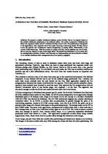
Figure 1. Problems in distributing the FMM across two nodes. Left: lightly-shaded boxes are on node 1 (Partition I) and darkly shaded boxes are on node 2 (Partition II). The thick line indicates the partition boundary line and the dash line shows the source points in both partitions needed by Partition II. The hashed boxes are in Partition I but they have also to be included in Partition II to compute the local direct sum. Right: light boxes belong to Partition I and dark boxes belong to Partition II. The multipole coefficients of the box with thick lines (center at C) is incomplete due to one child box on another node. Hence its parents (B and A) in the tree up to the minimal level are all incomplete.
small neighborhood domain of the evaluation point Ω(yj ) X X φ(yj ) = qi Φ(yj −xi )+ qi Φ(yj −xi ), (2) xi 6∈Ω(yj )
xi ∈Ω(yj )
in which the near-field sum is evaluated directly. The farfield sum is approximated by using kernel expansions and translations using a construct from computational geometry called “well separated pair decomposition” (WSPD) with the aid of recursive data-structures based on octrees (which usually have a construction cost of O(N log N )). There are several different versions of distributed FMM algorithms in the literature, such as [4], [5], [6], [7], [8], [9]. The basic idea is to divide the whole domain into spatial boxes and assigned them to each node in a way that the work balance can be guaranteed. To obtain correct results with such a data distribution several issues have to be accounted for (Fig. 1). The first is domain overlap: while receiver data points can be mutual exclusively distributed on multiple nodes, source data points which are in the boundary layers of partitions need to be repeated among several nodes for the near-field sum. The correct algorithm should not only determine such overlap domains and distribute data
5
7
13
15
4
6
12
14
1
3
9
11
0
2
8
10
12
Figure 2. Non-uniform domain distribution. Each node has the boxes with the same color. Here the box labeled as 12 needs box data from white, light gray and dark gray regions. It also has to distribute its data to those regions.
efficiently but also guarantee that such repeated source data are only translated once among all nodes. The second issue is incomplete translations, i.e. complete stencils may require translation coefficients of many boxes from other nodes. Thirdly, when source or receiver data points are distributed non-uniformly, the number of boxes assigned to each node may be quite different and the shape of each node’s domain and its boundary regions may become irregular. Such divisions require inter-node communication of the missing or incomplete spatial box data of neighborhoods and translations among nodes at all the octree levels (Fig. 2). Given the fact that no data from empty boxes are kept, it is challenging to efficiently determine which boxes to import or export data for all the levels. In the literature, distributed FMM and tree code algorithms commonly use the local essential tree (LET [9], [10]) to manage data exchange among all the computing nodes. Implementation details for import or export data via LETs are not explicitly described in the well known distributed FMM papers, such as [8], [9], [11], [12]. Recently, [1] developed a distributed FMM algorithms for heterogeneous clusters. However, their algorithm repeated part of translation computations among nodes and required coefficients exchange of all the spatial boxes at the octree’s bottom level. Such a scheme works well for small and middle size clusters but is not scalable to large size clusters. In another very recent work [13], the homogeneous isotropic turbulence in a cube containing 233 particles was successfully calculated, using a highly parallel fast multipole method (FMM) using 2048 GPUs, but the global communication of all the LETs is the performance bottleneck. In this paper, our purpose is to provide our new data structures and algorithms with implementation details to address the multiple node data management issues. A. Present contribution Starting from [1], we design a new scalable heterogeneous FMM algorithm, which fully distributes all the translations among nodes and substantially decreases its communication
costs. This is a consequence of the new data structures which separate the computation and communication to avoid synchronization during GPU computations. The data structures are similar to the LET concept but use a master-slave model and further have a parallel construction algorithm, in which the granularity is spatial boxes (which allows finer parallelization than at the single node level). Basically, each node divides its assigned domain into small spatial boxes via octrees and classifies each box into one of five categories in parallel. Based on the box type, each node determines the boxes that need to import and export data so that it would have the complete translation data after one communication step with the master. This can be computed on the GPU at negligible cost and this algorithm can handle non-uniform distributions with irregular partition shapes (Fig. 2). Our distributed algorithm improves timing results of [1] substantially and can be applied to large size clusters based on the better strong and weak scalability demonstrated. On our local Chimera cluster, we can perform a N -body sum for 1 billion particles on 32 nodes in 12.2 seconds (with the truncation number p = 8). II. T HE BASELINE FMM A LGORITHM In the FMM, the far-field term of Eq. 2 is evaluated using the factored approximate representations of the kernel function, which come from local and multipole expansions over spherical basis functions and are truncated to retain p2 terms. This truncation number p is a function of the specified tolerance ε = ε(p). Larger values of p result in better accuracy, but also increase computational time. The WSPD is recursively performed to subdivide the cube into subcubes via an octree until the maximal level lmax , or the tree depth, is achieved. The level lmax is chosen such that the computational costs of the local direct sum and far field translations can be balanced, i.e. roughly equal. The baseline FMM algorithm consists of four main parts: the initial expansion, the upward pass, the downward pass and the final summation. 1) Initial expansion: a) At the finest level lmax , all source data points are expanded at their box centers to obtain the farfield multipole or M-expansions {Cnm } over p2 spherical basis functions. The truncation number p is determined by the required accuracy. b) M-expansions from all source points in the same box are consolidated into a single expansion. 2) Upward pass: For levels from lmax to 2, Mexpansions for each child box are consolidated via multipole-to-multipole (M2M) translations to their parent source box. 3) Downward pass: For levels from 2 to lmax , local or L-expansions are created at each receiver box a) Translate M-expansions from the source boxes at the same level belonging to the receiver
Global Data Structure (K trees, roots at level 2)
Master Node
Slave Node
1
2
K Level 2
merge local octrees distribute the partition data
compute and send the local octree receive partition data
Level 3
exchange particle data
exchange particle data
Level 5
upward translations local summation
Level 4
Partitioning (K+L trees, roots at any level)
upward translations
exchange manager collect/distribute data
send/receive translation data
downward translations
downward translations
1
2
K Level 2
K+1
local summation
K+2
Level 3 Level 4
K+L
Level 5
Figure 4. Global data structure with K trees with roots at level 2 and partitioned data structure with roots at any level. Figure 3. An overview of the distributed FMM algorithm. Hashed parts are the overheads. Light and dark gray parts represent the kernel evaluation. GPU processes light gray part while CPU computes dark gray part.
box’s parent neighborhood but not the neighborhood of that receiver itself, to L-expansions via multipole-to-local (M2L) translations and consolidate the expansions. b) Translate the L-expansion from the parent receiver box center to its child box centers (L2L) and consolidate expansions. 4) Final summation: Evaluate the L-expansions for all receiver points at the finest level lmax and performs a local direct sum of nearby source points. The evaluations of the nearby source point direct sums are independent of the far-field expansions and translations, and can be performed separately. The costs of near-field direct sum and the far-field translations must be balanced to achieve optimal performance. Several different bases and translation methods have been proposed for the Laplace kernel. We used the expansions and methods described in [14], [15] and do not repeat details. Real valued basis functions that allow computations to be performed recursively with minimal use of special functions, or large renormalization coefficients are used. L- and M-expansions are truncated to retain p2 terms given the required accuracy. Translations are performed using the RCR decomposition. III. D ISTRIBUTED H ETEROGENEOUS FMM A LGORITHM Our distributed algorithm (Fig. 3) has five main steps : 1) Source and receiver data partition: a partition of the whole space that balances the workload among the computing nodes based on a cost estimation; it also handles overlapped neighborhoods. 2) Upward evaluation: each node performs initial Mexpansions of source points, upward translations and computes its own export/import box data.
3) Multiple node data exchange: we build a data exchange manager, which collects, merges and then distributes data from and to all nodes. 4) Downward evaluation: each node performs the downward pass and final L-expansions of its receiver points. 5) Local direct sum: each node performs this evaluation independent of the translations. The costs of partitions in Step (1) depend on the applications. For example, in many dynamics problems, from one time step to the next, it is very likely that most particles still reside on the same node, in which case the new partition may only require a small data exchange. In this paper, however, we assume the worst case that all data is assigned initially on each node randomly, which involves a large amount of particle data exchange. Based on the conclusion of [1], we perform Step (5) on the GPU, while Steps (2)–(4) are performed on the CPU in parallel. A. Distributed data structures The FMM data structure is based on data hierarchies for both sources and receivers; Figure 4 shows one. This can be viewed as a forest of K trees with roots at level 2 and leaves at level lmax . In the case of uniform data and when the number of nodes K ≤ 64 (for the octree) each node may handle one or several trees. If the number of nodes is more than 64 and/or data distributions are substantially nonuniform, partitioning based on the work load balance should be performed by splitting the trees at a level > 2. Such a partitioning can be thought of as breaking of some edges of the initial graph. This increases the number of the trees in the forest, and each tree may have a root at an arbitrary level l = 2, ..., lmax . Each node then takes care for computations related to one or several trees according to a split of the workload. We define two special octree levels: •
Partition level lpar : At this level, the whole domain is partitioned among different nodes. Within each node,
i
e
partition module distributes inputs: particle positions, source strength
E I
d R o
Figure 5. An example of source box types. White boxes are Partition I and gray boxes are Partition II. The partition level is 3 and the critical level is 2. Solid line boxes correspond to level 2 and dash line boxes correspond to level 3. At partition II, box e and E are export boxes. Boxe i and I are import boxes. Box R is a root box. Box d is a domestic box. Box o is an other box.
•
all the subtrees at this level or below are totally complete, i.e., no box at level ≥ lpar is on other nodes. Critical level lcrit = max (lpar − 1, 2): At this level, all the box coefficients are broadcasted such that all boxes at level ≤ lcrit can be treated as local boxes, i.e., all the box coefficients are complete after broadcasting.
Note that the partition level is usually quite low for 3D problems, e.g., lpar = 2, 3, 4, therefore only a small amount of data exchange is needed to broadcast the coefficients at the critical level lcrit . To manage the data exchange, we classify source boxes at all levels into five types. For any node, say J, these five box types are: 1) Domestic Boxes: The box and all its children are on J. All domestic boxes are organized in trees with roots located at level 1. All domestic boxes are located at levels from lmax to 2. The roots of domestic boxes at level 1 are not domestic boxes (no data is computed for such boxes). 2) Export Boxes: These boxes need to send data to other nodes. At lcrit , the M-data of export boxes may be incomplete. At level > lcrit , all export boxes are domestic boxes of J and their M-data are complete. 3) Import Boxes: Their data are produced by other computing nodes for importing to J. At lcrit , the Mdata of import boxes may be incomplete. At level > lcrit , all import boxes are domestic boxes of nodes other than J and their M-data are complete there. 4) Root Boxes: These are boxes at critical level, which need to be both exported and imported. For level > lcrit there is no root box. 5) Other Boxes: Boxes which are included in the data structure but do not belong to any of the above types,
ODE solver: source and receiver update
data structures (octree, neighbors, source box types) source M-expansions
translation stencils upward translations
local summation
translation data exchange downward translations
receiver L-expansions final summation
Figure 6. The distributed FMM algorithm. The hashed part are the data partition module. The light gray parts of the algorithm is computed by using the GPU while dark gray parts are computed by using the CPU. Double ended Arrows represent the communication with other nodes. The rectangle with dash lines represents the parallel region.
e.g. all boxes of level 1, and any other box, which for some reason is passed to the computing node (such boxes are considered to be empty and are skipped in computation, so that affects only the memory and amount of data transferred between the nodes). Refer Fig. 5 for an example. Note that there are no import or export boxes at levels from lcrit − 1 to 2. All boxes at these levels are either domestic boxes or other boxes after the broadcast and summation of incomplete M-data at lcrit . In our algorithm, we only need compute M-data and box types from level lmax to lcrit and exchange the information at lcrit . After that we compute the M-data for all the domestic boxes up to level 2 then produces L-data for all receiver boxes at level lmax handled by the computing node. B. The distributed FMM algorithm In our FMM algorithm, all the necessary data structures, such as octree and neighbors, and particle related information, are computed on the GPU using the efficient parallel methods presented in [1], [16]. Details of the algorithms and implementations are not reported here. Given the global partition, how the algorithm appears on a single node is illustrated in Fig. 6. Assume that all the necessary data structures for the translations, such as box’s global Morton indices, the neighbor, export/import box type lists and those initial M-expansion data, are available, then each node J
MASTER NODE
MANAGER
SLAVE NODE
UPWARD
AT CRITICAL LEVEL
DOWNWARD
Figure 7. A simple multiple node 2D FMM algorithm illustration (lcrit = 2) : the top rounded rectangular is the MASTER NODE which is also chosen as the data exchange manager. The bottom rounded rectangular is the SLAVE NODE. From left to right is how the algorithm proceeds. Each node perform upward M-translations from lmax to lcrit . At critical level the manager collect and distribute data from and to all the nodes. Those isolated boxes in this figure are import/export boxes. After this communication with master, all the nodes perform downward M2L and L2L translations only for its own receiver boxes.
executes the following translation algorithm: 1) Upward translation pass: a) Get M-data of all domestic source boxes at lmax from GPU global memory. b) Produce M-data for all domestic source boxes at levels l = lmax − 1, . . . , max(2, lcrit ). c) Pack export M-data, the import and export box indices of all levels. Then send them to the data exchange manager. d) The master node, which is also the manager, collects data. For the incomplete root box Mdata from different nodes, it sums them together to get the complete M-data. Then according to each node’s emport/import box indices, it packs the corresponding M-data then sends to them. e) Receive import M-data of all levels from the data exchange manager. f) If lcrit > 2, consolidate S-data for root domestic boxes at level lcrit . If lcrit > 3, produce Mdata for all domestic source boxes at levels l = lcrit − 1, . . . , 2. 2) Downward translation pass: a) Produce L-data for all receiver boxes at levels l = 2, . . . , lmax . b) Output L-data for all receiver boxes at level lmax . c) Redistribute the L-data among its own GPUs. d) Each GPU finally consolidates the L-data, add the local sums to the dense sums and copy them back to the host according to the original inputting receiver’s order. Here all boxes mean all boxes handled by each node. A simple illustration of this algorithm for a 2D problem is shown in Fig. 7.
Algorithm 1 Compute source box type on the node J Input: a source box index BoxIndex[i]= k at level l Output: BoxType[i] isOnNode←isImportExport←isExport←FALSE if l