1
Scalable Feature Extraction for Coarse-to-Fine JPEG 2000 Image Classification Antonin Descampe*, IEEE Member, Christophe De Vleeschouwer, IEEE Member, Pierre Vandergheynst, IEEE Member, and Benoit Macq, IEEE Fellow.
Abstract In this paper, we address the issues of analyzing and classifying JPEG 2000 code-streams. An original representation, called integral volume, is first proposed to compute local image features progressively from the compressed code-stream, on any spatial image area, regardless of the codeblocks borders. Then, a JPEG 2000 classifier is presented, that uses integral volumes to learn an ensemble of randomized trees. Several classification tasks are performed on various JPEG 2000 image databases and results are in the same range as the ones obtained in the literature with noncompressed versions of these databases. Finally, a cascade of such classifiers is considered, in order to specifically address the image retrieval issue, i.e. bi-class problems characterized by a highly skewed distribution. An efficient way to learn and optimize such cascade is proposed. We show that staying in a JPEG 2000 framework, initially seen as a constraint to avoid heavy decoding operations, is actually an advantage as it can benefit from the multi-resolution and multi-layer paradigms inherently present in this compression standard. In particular, unlike other existing cascaded retrieval systems, the features used along our cascade are increasingly discriminant and lead therefore to a better complexity vs performance trade-off.
EDICS: ARS-SRE Image & Video Storage and Retrieval, COM-LOC Lossy Coding of Images & Video A. Descampe, C. De Vleeschouwer, and B. Macq are with the Communications Laboratory (TELE), Louvain School of Engineering (EPL), UCL, Place du Levant, 2, 1348 Louvain-la-Neuve, Belgium (e-mail: {antonin.descampe, christophe.devleeschouwer, benoit.macq}@uclouvain.be). P. Vandergheynst is with the LTS2 laboratory, Electrical Engineering Institute, EPFL, ELB 111 (Building ELB) Station 11, CH - 1015 Lausanne Switzerland (e-mail:
[email protected]). This work has been partly funded by the Walloon Region (FirstPostDoc MOSAIC) and the Belgian NSF (F.R.SFNRS).
January 27, 2011
DRAFT
2
I. Introduction Today’s imaging applications have to deal with an ever-growing amount of digital data. Management and exploitation of this information requires (1) an efficient and flexible representation of the images, and (2) application-specific techniques exploiting this flexibility to guide and assist the user in his search in the data space. Such techniques could be useful in any application that involves (semi-)automatic image categorization or retrieval tasks, such as audiovisual archives retrieval, computer-assisted medical diagnosis, remote sensing on satellite images, etc. In this paper, we focus on a compressed scalable image representation, namely JPEG 2000, and investigate how discriminant features can be extracted from such embedded code-stream to perform image categorization and retrieval tasks. Being able to search for relevant images directly within compressed bit-streams (or through a partial decompression) has an obvious advantage in terms of computational load. Moreover, we show in this paper that JPEG 2000 is actually well suited for image retrieval tasks. Indeed, its various scalability levels allow for true and efficient coarse-to-fine searches among the bit-streams. Furthermore, the JPEG 2000 wavelet transformation has also a strong discriminant power and is suited to analyze image characteristics like edges and textures. Among the broad range of imaging applications involving classification or retrieval tasks, we will focus on those where areas of interest are characterized by an ensemble of different textures. Texture has to be understood here in the broad sense of a “set of local neighbourhood properties of the gray levels of an image region” [1]. “Grays levels” is even too restrictive in our case as color information (at least in the low frequencies) will also be exploited in the retrieval process. While this choice might appear to exceedingly narrow the set of potential applications, we will show that many objects can actually be characterized by an ensemble of textures. This is even truer if the relative spatial positions of the textures composing an object are taken into account, as it will be the case in the proposed system. Focusing on texture-based retrieval techniques, we will not consider shape matching algorithms, like the ones presented (in a JPEG 2000 framework) in [2]. However, these algorithms could efficiently complement the proposed retrieval system and are, as such, an interesting future research direction. II. Overview Figure 1 presents an overview of the proposed system. Its goal is to determine if an image, stored in the JPEG 2000 format, is similar to a set of images of interest. Practically, for each image that has to be analyzed, discriminant features are extracted from its JPEG 2000 code-stream. Several January 27, 2011
DRAFT
3
successive features sets are extracted, each one with an extraction cost slightly higher than the previous one, but also with a potentially higher discriminant power. A first classifier uses the first features set, and feeds a second classifier with the processed images that are likely to be positive. The second classifier uses the two first features sets and passes the image to the third classifier if needed and so on. If an image is very different from the image(s) of interest, it will be identified as such very early in the procedure and will be quickly discarded. On the contrary, a relevant image will pass the successive classifiers and reach the end of the cascade. By doing so, the amount of data that has to be decoded from the JPEG 2000 code-stream is directly related to the relevance of the image. We show in this paper that JPEG 2000 is particularly well suited for this kind of coarse-to-fine classification.
Contribution 1: integral volume feature extraction
J2K code-stream
Progressive decoding (as long as not rejected by a classifier) Feature granularity
coarse
Features set 1
Classifier 1 p1 ⩼ θ1
Features set 2
true
Classifier 2 p2 ⩼ θ2
true
fine
...
Features set n
...
Classifier n pn ⩼ θn
false
false
true
If this point is reached => positive sample
false
If this point is reached => negative sample
Contribution 2: randomized tree classifier design
Fig. 1.
Contribution 3: cascade of classifiers with optimized performance vs complexity trade-off
System overview. Starting from a JPEG 2000 image, discriminant features are progressively extracted from
it and feed a cascade of classifiers. As long as the image is not considered as negative by the cascade, each classifier i will compute a probability pi that the image is positive and compare it to a threshold θi (i = 1, .., N ).
January 27, 2011
DRAFT
4
A. Contributions Three main contributions are presented in this paper. We now introduce each of these ideas briefly and describe them in details in subsequent sections. The first contribution is a method to extract, process and store a hierarchy of features from a JPEG 2000 code-stream. Both header-based [3] and wavelet-based [2] features are considered. To store all the extracted JPEG 2000 features values, we extend the concept of integral image first introduced in [4] and more recently made famous by Viola and Jones in [5]. We propose to represent a JPEG 2000 code-stream with a chain of integral volumes. This representation draws benefit from the JPEG 2000 scalability levels and allows for a very fast features computation on any image area. The second contribution is the combination of integral volumes mentioned above with an ensemble of random decision trees [6] to build an efficient and robust JPEG 2000 image classifier. Based on the work by Mar´ee et al. [7], we take advantage of the integral volume structure to generate random samples in the images. We show that chosen features lead to satisfying classification results on several different image databases. The last contribution is the tight integration of the JPEG 2000 scalability levels for designing a cascade of JPEG 2000 image classifiers. Cascade of classifiers are well suited for image retrieval tasks and object detection. When one has to dig into a compressed image database, the challenge is to retrieve relevant areas while minimizing the amount of decompressed data. In this work, starting from the coarse classification that can easily be obtained from header-based features, we use the resolution and bit-depth scalability of JPEG 2000 to progressively extract more information and refine the classification as we go deeper into the cascade. For a given image area, the amount of data that will need to be entropy-decoded is therefore directly related to the relevance of this area in the retrieval process. This idea is directly inspired from the work of Geman and Fleuret [8] and from the one of Viola and Jones [5]. Concurrently to [9], we proposed in [10] to improve the Viola and Jones cascade by taking into account the extraction cost of a feature. This leads us to an interesting “complexity1 vs performances” trade-off when designing a cascade of classifiers. 1
This complexity being computed as the total amount of data that has to be decompressed in the retrieval process.
January 27, 2011
DRAFT
5
B. Paper organization The remainder of the paper is organized as follows. Section III first gives some JPEG 2000 key elements and then details which features are used and how they are extracted from JPEG 2000 code-streams. In particular, the scalability of the extraction process is underlined. We also introduce the concept of integral volume to store these features. In Section IV, integral volumes are combined with random decision trees to set up a JPEG 2000 classifier. Experiments on several widely used and publicly available datasets are presented, showing the discriminant power of our JPEG 2000 classifier. Then, in Section V, several of these classifiers are cascaded to address image retrieval problems in a computationally efficient way. Experiments on two well known datasets (namely the PONCE textures dataset [11] and the UKBENCH dataset [12]) are detailed to illustrate the effectiveness of the cascade approach. Finally, Section VI summarizes the paper and gives future research directions. III. Scalable feature extraction Numerous papers have been written on the use of JPEG 2000 code-streams for classification or retrieval tasks. Each of them proposes a set of features that can be more or less easily extracted from the code-stream and that is used in a classification process, most often based on some kind of distance metric. As we shall see, the proposed approach uses features with similar discriminant power than the ones proposed in the related literature. However, a significant contribution of our work compared to the existing literature is that we take advantage of the JPEG 2000 scalability to trade-off between the classification accuracy and the amount of data that has to be extracted from the code-stream. A. JPEG 2000 key elements We now review the elements of the JPEG 2000 compression standard that are relevant to understand the rest of the paper. Interested readers may refer to [13] for more details. In short, JPEG 2000 is based on successive dyadic discrete wavelet decompositions of the image components, whose subbands are partitioned into code-blocks that are coded independently. Each code-block is entropy-coded into an embedded bitstream, i.e. into a stream that provides a representation that is (close-to-)optimal in the rate-distortion sense when truncated to any desired length. This implies in particular that wavelet coefficients are coded bit-plane by bit-plane, from the Most Significant Bit (MSB) to the Least Significant Bit (LSB). January 27, 2011
DRAFT
6
Any JPEG 2000 code-stream is organized as a succession of packets, each packet containing data referring to a certain resolution, a certain image component, a certain spatial zone, and a certain range of bits inside the coefficients bit-depth (this last element is referred to as the SNR scalability). It is therefore possible to decode a JPEG 2000 code-stream in many different ways, without having to process all the packets. To obtain a low resolution version of the image for example, one has simply to extract the related low resolution packets. B. Feature types Two kind of features can basically be extracted from a JPEG 2000 code-stream: the ones from the packet headers that do not involve any partial decompression, and the ones based on the wavelet coefficients that require an entropy-decoding step. 1) Header-based features: as mentioned above, a JPEG 2000 code-stream is made of a succession of packets. Each packet has a header that contains relevant information about its content. In particular, for a given code-block present in a packet, we can extract B , the number of bytes used to entropically encode the image data contained in the code-block, and M , the maximum number of significant bit-planes1 in the code-block. The former reflects the efficiency with which the entropy coder did compress the wavelet coefficients from this code-block. As such, it can be seen as a measure of the source entropy and gives therefore a good indication on the informational content of the code-block [3]. The latter corresponds to the log2 of the maximum modulus of the wavelet coefficients present in the code-block. In [14], Mallat showed that this maximum modulus well describes the kind of singularity present in the image. It has been used for example in [15]. In terms of extraction complexity, these features are of great interest as they do not imply any (partial) entropic decompression of the JPEG 2000 code-stream. In the following, we will consider only the number of entropy-coded bytes B , as experiments have shown little improvement when using both kind of features. 2) Wavelet-based features: research on wavelet-based retrieval techniques has been ongoing for many years now. The spatial-frequency representation provided by the wavelet transform gives important information on the kind of local singularities present in the image. In particular, textures end edges are well discriminated based on the statistical properties of the wavelet coefficients 1
A significant bit-plane is a bit-plane which either contains at least one non-zero bit or is below another significant
bit-plane January 27, 2011
DRAFT
7
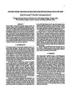
distribution. [16] proposes to model this distribution with a Generalized Gaussian Density (GGD) and hence, to characterize an image with the vector aggregating the 2 parameters of a GGD in each subband. [17] follows the same approach using Gaussian Mixture Models instead of GGD. Like in [16] and [17], we propose to characterize the probability distribution of the wavelet coefficients by a set of parameters. Starting from a JPEG 2000 code-stream, the extraction process of these parameters obviously implies an entropy-decoding step, as we have to get back to the wavelet coefficients. Unlike [16] and [17], a very simple distribution approximation is used: it does not require any computational overhead in addition to the decoding step and, more importantly, it can be progressively refined during the decoding step. Let’s consider a code-block with M significant bit-planes. As a bit-plane from this code-block is being decoded, new significant coefficients are counted. For a given bit-plane k (k = 1, ..., M ), the number Sk of new significant coefficients corresponds to the amount of wavelet coefficients x in the code-block such that 2k−1 ≤ |x| < 2k .
As illustrated in Fig. 2, these Sk (k = 1, ..., M ) values might be considered as the bin values of a non-uniform histogram. As such, they correspond therefore to an approximation of the wavelet coefficients distribution for the related code-block. In the following, we propose to use these bin values corresponding to the decoded bit-planes as independent wavelet features.
1000
800 600 400 200 0
0
1
2
3
(a)
4 k
5
6
7
8
1000 # of wavelet coefficients (Sk)
# of wavelet coefficients (Sk)
# of wavelet coefficients (Sk)
1000
800 600 400 200 0
0
1
2
3
(b)
4 k
5
6
7
8
800 600 400 200 0
0
1
2
3
4 k
5
6
7
8
(c)
Fig. 2. Example of progressive building of the wavelet coefficients histogram, during JPEG 2000 decompression. Bin k corresponds to the number of wavelet coefficients x such that 2k−1 ≤ |x| < 2k . S0 is the number of coefficients equal to zero. (a) Before decoding the first (most significant) bit-plane, no information is available on the coefficients distribution. (b) When decoding the five most significant bit-planes, the number of new significant coefficients is counted for each bit-plane and gives the first five bin values. (c) Complete histogram (all bit-planes decoded).
The header and wavelet-based features described above will be used to feed the proposed image January 27, 2011
DRAFT
8
classifier. As the application may require to compare (portions of) images that do not necessarily have the same amount of pixels, the values B and Sk are normalized by the total number N of coefficients present in the sample, to define b and sk , respectively. C. Scalable extraction The feature extraction process can take advantage of the scalability inherently present in JPEG 2000, namely the spatial, resolution and SNR scalability levels. It is indeed possible to make a trade-off between the desired characterization accuracy and the feature extraction cost it implies. Let’s consider a given spatial area in an image. The spatial scalability of JPEG 2000 allows to select the packets related to this area without having to process the remaining codestream. Then, a coarse characterization of the area content can be obtained by extracting the header-based features, from the lowest to the highest resolution. If a more accurate description of the image content is required, we can complement the header information with wavelet-based features, at the cost of an higher computation load (as entropy-decoding operations are required). The wavelet coefficient distribution is approximated, from the lowest to the highest resolution. Moreover, for each resolution, this approximation is progressively refined as more bit-planes are decoded (using the SNR scalability). To illustrate the benefit that can be drawn from such scalable extraction, a texture classification process is presented. Let’s consider 4 different classes of textures. Each class contains 40 items, each one being a 640x480 grayscale image. Samples from each class are presented in Fig. 3a. All images are JPEG 2000-compressed with 4 resolution levels, resolution 1 corresponding to the lowest resolution (the LL-subband). There are three successive steps in this example of classification process, each using a bit more information than the previous one. In the first step of the classification process, only very cheap features are used, namely headerbased features. As we see on Fig 3b, this information is already sufficient to discriminate the “water” class from the three other ones. For the second step, in addition to the header information, we now assume that the 2 most significant bit-planes (7th and 8th) of resolution 1 and 2 have been decoded. As shown in Fig. 3c, this new information allows to clearly separate the “glass2” samples from the two remaining classes, although it was not possible to do so with header-based features only. In the last step, the third most significant bit-plane (the 6th) from all resolutions is supposed to be decoded. Fig 3d shows how the two last classes can be separated.
January 27, 2011
DRAFT
9
0.8
0.75
0.7
0.65 nmq 4
b4
0.6
0.55
water glass1 glass2 corduroy
0.5
0.45 0.7
0.75
0.8
0.85 nbmq 2
0.9
0.95
1
2
(a)
(b)
0.25
0.1
glass1 glass2 corduroy
glass1 corduroy
0.09
0.2
0.08 0.07
0.15 nsc 7; 2
0.06
s7,2
nsc 6; 4
s6,4 0.05 0.1
0.04 0.03
0.05
0.02 0.01
0
0
0.1
0.2
0.3
sc sn7,1 7;1
(c)
0.4
0.5
0.6
0.7
0
0.2
0.25
0.3
sc sn6,1 6;1
0.35
0.4
0.45
0.5
(d)
Fig. 3. A scalable classification process. (a) Texture samples randomly selected from 4 different classes, one in each row: water, glass1, glass2 and corduroy. Source : Ponce texture database [11]. (b) The first step uses only header information and is able to discriminate the “water” class from the three other ones. (bi = normalized number of entropy-coded bytes for resolution i). (c) In the second step, the two most significant bit-planes from resolution 1 and 2 have been decoded and allow to separate textures from class “glass2”. (sj,i = fraction of new sign. coeff. in bp j, for res. i). (d) The third and final step allows to more clearly discriminate the two remaining classes, “glass1” and “corduroy”.
January 27, 2011
DRAFT
10
As we see, this scalable extraction perfectly fits with a classification process made of several cascaded classifiers. This will be detailed in Section V and used in an image retrieval context. D. Integral volume representation Let’s summarize what we do have up to this point. Considering a code-block c of a JPEG 2000 compressed image, the relevant information that can be extracted about it is (i) bc , the normalized number of bytes used to entropically encode code-block c, and (ii) sk,c , the fraction of code-block coefficients that become significant in the bit-plane k (k = 1, .., Mc ). Each of these extracted values gives a global information on the code-block. If the area of interest is made of several code-blocks, these values are very simply aggregated. A drawback of the features described above is that we have to stick to code-blocks borders when selecting an area of interest. All code-blocks in a JPEG 2000 code-stream have indeed the same size, which is typically around 32x32 or 64x64 pixels. At low resolution levels, such amount of pixels can cover a very large spatial area, which can reveal itself to be very constraining if we want to extract relevant information from a smaller spatial zone. To solve this problem and extract features very rapidly, on any spatial area, independently from code-blocks borders, we propose an intermediate representation of the image, called integral volume. This representation is a direct extension of the integral image introduced in [4] and more recently made famous in [5]. Starting from an image P where P (i, j) is the pixel value at coordinates (i, j), the integral image IP is defined as X
IP (i, j) = 0
P (i0 , j 0 )
(1)
0
i ≤i,j ≤j
Having computed this integral image IP allows to very quickly compute the sum of all pixel values in any rectangular area contained in P [5]. Let (ir , jr ) denote the coordinates of the top-left corner of a given rectangle r in P , and w and h the width and height of r. The sum of pixels SP,r in rectangle r is simply given by SP,r = IP (ir , jr ) + IP (ir + w, jr + h) − IP (ir + w, jr ) − IP (ir , jr + h)
(2)
In this paper, we propose to use, for each bit-plane k from each code-block c, the integral image concept described above, where the matrix of pixel values P has been replaced by the significance
January 27, 2011
DRAFT
11
map σk,c (i, j): σk,c (i, j) = 1 =0
if c(i, j) ≥ 2k−1 otherwise.
where c(i, j) refers to the coefficient value at coordinates (i, j) in code-block c. By doing so, we s such that each element T s (i, j) at column i and row j is the number of obtain a table Tk,c k,c
significant coefficients in code-block c at bit-plane k , among all coefficients above and to the left of element (i, j), inclusive: X
s Tk,c (i, j) =
σk,c (i0 , j 0 ) , for i = 1, ..., Wc and j = 1, ..., Hc
i0 ≤i,j 0 ≤j
where Wc and Hc are respectively the width and height of code-block c. s perfectly fits with the entropy-decoding procedure of Interestingly, computation of table Tk,c
bit-plane k . Indeed, the significance status of each coefficient of a code-block is a state variable of the JPEG 2000 entropy decoder. As such, it is constantly maintained and updated during the decoding procedure. Hence, once bit-plane k has been decoded, σk,c (i, j) is directly available and s (i, j) is obtained by the following recursive formula Tk,c s s s s Tk,c (i, j) = Tk,c (i − 1, j) + Tk,c (i, j − 1) − Tk,c (i − 1, j − 1) + σk,c (i, j).
Initial conditions are set based on the previously decoded adjacent code-blocks, as shown in Fig. 4. s related to the whole subband sb. Hence, we obtain an integral table Tk,sb
0
1
0
0
0
1
0
15
18
20
21
21
24
25
1
1
1
1
0
0
1
19
23
26
28
28
31
33
0
1
0
1
1
0
0
20
25
28
31
32
35
37
1
0
0
1
0
1
0
23
28
31
35
36
40
42
0
0
0
0
0
1
1
24
29
32
36
37 42
45
0
1
1
0
1
0
0
24
30
34
38
40
45
48
1
1
0
1
1
1
0
27
34
38
43
46
52
55
sc Fig. 4. Integral table Tk,c with adjacent code-blocks taken into account. Initial conditions are set to the border lines
values of the code-block currently decoded (black bold numbers in the figure).
s By stacking the tables Tk,sb for all bit-planes of subband sb, we obtain what we call an integral
January 27, 2011
DRAFT
12
volume of this subband. Each element of such volume is simply given by s Vsb (i, j, k) = Tk,sb (i, j) f or i = 1, ..., Wsb
(3)
j = 1, ..., Hsb k = 1, ..., Msb
where Wsb and Hsb are respectively the width and height of subband sb. Msb is the maximum number of bit-planes in the subband. Once computed, this integral volume allows to easily obtain the normalized number sA,K of new significant coefficients in bit-plane range K (K = [k0 ; k1 ], k0 ≤ k1 ), on any spatial area A, defined by its upper left corner (i0 , j0 ) and its lower right corner (i1 , j1 ), inside the subband sb: sA,K
(4)
= (Vsb (i0 , j0 , k0 ) + Vsb (i1 , j1 , k0 ) −Vsb (i0 , j1 , k0 ) − Vsb (i1 , j0 , k0 ) −Vsb (i0 , j0 , k1 ) − Vsb (i1 , j1 , k1 ) +Vsb (i0 , j1 , k1 ) + Vsb (i1 , j0 , k1 )) / (i1 − i0 ) . (j1 − j0 ) .
In order to have a single representation from which it would be possible to extract both wavelet and header-based features, we use the same concept of integral table to store the bc values (defined on page 10). Assuming that any coefficient belonging to code-block c is encoded using βc =
Bc Wc .Hc
bytes per coefficient, we define the integral table Tcb as Tcb (i, j) = Tcb (i − 1, j) + Tcb (i, j − 1) − Tcb (i − 1, j − 1) + βc (i, j) s , table T b can be extended to T b related to the whole for i = 1, ..., Wc and j = 1, ..., Hc . Like Tk,c c sb b on top of all tables T s subband. By adding table Tsb k,sb of the integral volume Vsb defined in Eq. 3,
the normalized number of bytes used to encode all coefficients in area A is given by: bA = (Vsb (i0 , j0 , Msb + 1) + Vsb (i1 , j1 , Msb + 1)
(5)
−Vsb (i0 , j1 , Msb + 1) − Vsb (i1 , j0 , Msb + 1)) / (i1 − i0 ) . (j1 − j0 ) .
Eventually, to increase the robustness to rotation changes, integral volumes from the 3 different subbands of a same resolution level are merged by an averaging operation: P Vsb (i, j, k) Vr (i, j, k) = sb 3
January 27, 2011
DRAFT
13
In conclusion, starting from any JPEG 2000 image, compressed with NL decomposition levels, an intermediate representation called integral volume can be progressively built, as more data is decompressed. It consists in several different volumes of size Wr xHr x(Mr + 1) (r = 0, .., NL ). With this data structure available, one can easily get the normalized number of bytes bA,r used to encode a spatial area A in resolution r, and the normalized number of new significant coefficients sA,K,r for a range of bit-planes K inside resolution r of spatial area A . IV. A JPEG 2000 image classifier In our work, we propose to combine an ensemble of random decision trees with our JPEG 2000 integral volume representation. Tree-based methods consist in a succession of answers to (binary) questions that progressively divide (and classify) an initial set of items [18]. Randomization [19], when applied to decision trees, can drastically reduce the variance and overfitting problems generally affecting decision trees [6]. The design of our image classifier involves three successive steps that we detail hereunder. A. Method 1) Sampling: we define a sample as the basic element that will be classified by the ensemble of random decision trees. An entire image could be considered as a single sample but it appears that subsampling images has several advantages when dealing with classification tasks. The main one is that it increases the robustness of the classifier: all samples from an image do not need to be correctly classified to still make a good decision about the class of the image. Like in [7], the subsampling operation consists in selecting square subwindows of random sizes and at random positions. Thanks to the integral volume representation described above, the subsampling operation only consists in randomly generating pairs of coordinates, each pair corresponding to the upper left and lower right corners of a sample. Then, once a sample has been defined inside the image, feature values bA,r or sA,K,r are extracted from it by specifying a resolution r, a bit-plane range K and a spatial zone A inside the sample, as described at the end of previous section. Unlike [7],
there is no “fixed-size feature vector” characterizing each sample. Actually, there is virtually an unlimited number of features that can be extracted from a given sample. 2) Learning: During the learning phase, samples from the learning set are used to train an ensemble of extremely randomized trees [6] (Extra-Trees). In an ensemble of T Extra-Trees, candidate splits are chosen completely at random. This means that both the tested feature and the January 27, 2011
DRAFT
14
cut point selected for thresholding, are chosen randomly. The split eventually chosen is either the best one among K candidates, or the first one to reach a minimum score Scmin . The score measure is based on the entropy reduction brought by the split. The splitting process is repeated recursively until a node contains less than nmin samples. A leaf l from a tree t is then characterized by a probability distribution pt (i|l) (i = 1, ..., nc ), the probability that a sample reaching leaf l belongs to the ith class among nc classes. This distribution is simply obtained by counting, for each class, the training samples reaching this leaf. 3) Testing: During the test step, Ntest samples are extracted from each test image and are propagated in the T trees. Each sample reaches a specific leaf in each tree. Once all Ntest samples from the test image k have been propagated in the T trees, we obtain a set Lk = {lk } of reached leaves on image k . The probability p(i|Lk ) that image k belongs to class i is estimated by PT 1 X t=1 pt (i|lk ) p(i|Lk ) = Ntest T lk ∈Lk
and the class
c∗k
predicted for test image k is simply c∗k = arg max p(ck |Lk ). ck ∈[1;nc ]
B. Experiments Several experiments have been conducted to assess our image classifier and analyze the discriminant power of the JPEG 2000 features introduced in Section III. It should be noted that no complexity or speed considerations are envisioned in these experiments. These aspects are investigated in Section V, where the JPEG 2000 scalability is exploited to achieve a coarse-to-fine image classification. Following parameters for the ensemble of random decision trees have been used (see Section IV-A2 for the meaning of these parameters): T = 10, K = 30, nmin = 2 (which means that the trees are fully grown), Scmin = 0.25. During the learning phase, a total of 100 000 samples have been extracted from the learning images while during the test phase, 100 samples have been computed in each test image to decide to which class this image belongs. We invite the reader to refer to [6] for a deeper analysis of the influence of each of these parameters. Six databases have been used: PONCE [11], ZUBUD [20], ETH-80 [21], COIL-100 [22], CALTECH101 [23] and CALTECH256 [24]. These datasets, the experiments protocols and the JPEG 2000 compression parameters are summarized in Appendix on page 28. For the COIL-100 dataset, two different protocols have been used. Table I compares our performances to other results. January 27, 2011
DRAFT
15
In particular, we focus on the system proposed in [7]. Our system mainly differs from [7] in the fact that features are extracted from a compressed code-stream and not from the pixel-domain. Consequently, the comparison to such system should give us a good indication on the analysis capacity that JPEG 2000 can offer in a classification task. TABLE I Classification error rates achieved by the system extracting Random Subwindows (“RSw”) from the uncompressed images (“Raw”), described in [7], and by our system. The best other result found in the literature is indicated in the last column. Raw + RSw
Ours
Others
PONCE
45.20%
11.20%
-
ZUBUD
4.35% [7]
4.35%
0% [25]
ETH-80
25.49% [7]
19.02%
13.6% [21]
COIL-100 (1)
13.58% [7]
22.51%
24% [25]
COIL-100 (2)
0.5% [7]
0.17%
0.1% [25]
CALTECH101
62.9%
53.9%
18.7% [26]
CALTECH256
92.9%
88.7%
54.7% [26]
Compared to the system based on random subwindows extracted from uncompressed images, the results obtained with our classifier (JPEG 2000 compression and integral volume extraction) are always equal or better, except for “COIL-100 (1)” experiment. This tends to prove the higher discriminant power of wavelet histogram bins compared to averaged pixel values. In particular, the error-rates obtained for the PONCE dataset underline the higher ability of the proposed JPEG 2000 classifier to discriminate textures. Concerning the “COIL-100 (1)” experiment, the result illustrates the lack of robustness of the proposed classifier in presence of viewpoint changes. Wavelet histogram bins are more sensitive to a viewpoint change than average pixel values. Compared to other results in the literature, the performances achieved by our system are always close to the best result, except for the CALTECH datasets. This can be explained by the lack of robustness of our features against the intra-class variability of CALTECH datasets. As long as this intra-class variability is reasonable (for example each class being populated with pictures of the same object with orientation and lightning changes), simple and easy-to-compute features like in [7] and ours are sufficient to achieve good classification performance, while keeping a low computational load (see Section V-B page 18 for a quantitative analysis of the computational January 27, 2011
DRAFT
16
efficiency of our system). When the intra-class variability gets higher (each class being populated with pictures of different scenes representing the same semantic concept), like in CALTECH101 and even more in CALTECH256, more sophisticated sampling procedures and more discriminative features are required. These could be based on the spatial pyramid matching algorithm proposed in [27], the SVM-kNN algorithm in [28] or the combination of region-of-interest identification, shape and appearance descriptors, and random forests, as proposed in [26]. It should be noted that such more elaborated features could also be extracted from JPEG 2000 code-streams and would mainly imply a computation overhead when processing integral volumes. V. Coarse-to-fine image classification: a cascade of image classifiers In this Section, we consider a typical image retrieval problem, for which there are only two classes (positive and negative images) that are highly asymmetric (there are much more negative images than positive ones). We exploit the JPEG 2000 scalability, to limit as much as possible the amount of information that has to be partially decompressed when searching a large dataset. A. Cascading classifiers To take into account the class asymmetry, a natural idea that comes up is to first try to reject the most obvious negative images rather than trying to find directly the few positive events. In this way, we are left with our positive images disseminated in a much smaller amount of negative ones. Of course, this subset of images is harder to discriminate but as it is much smaller, we can afford to spend more computational load on each of its images. This simple idea has lead to the cascade of classifiers concept [5], [8]. As shown in Fig. 1 on page 3, a cascade of classifiers is made of a succession of stages, each of them being fed by the images identified as positive by the previous stage. For a given image, each stage i will compute a probability pi that the image is positive and compare it to a threshold θi . Formally, an image retrieval system has two objectives: maximize the detection rate and minimize the false positive rate. Such cascade framework allows to relax the latter one. Indeed, if a negative image is accepted, next stages still have the opportunity to reject it. The succession of stages will then guarantee a small global false positive rate, by multiplying the succession of moderate intermediate false positive rate. The concept of cascading classifiers is not new and has already been investigated in the literature. Among others, Viola and Jones proposed a cascade of boosted classifiers based on simple rectangle
January 27, 2011
DRAFT
17
features for robust real-time object detection [5]. Each stage is a weighted sum of single-featurethresholding classifiers, trained through an AdaBoost process. In a more recent work [29], Brubaker et al. questioned the relevance of single-feature-thresholding classifier and showed that the overall performance could benefit from stronger weak classifiers like CART (Classification And Regression Trees). In our work, we push this idea one step further by using an ensemble of random decision trees for each stage. Such random decision tree is a stronger weak classifier than thresholding on a single feature, but is also much easier and faster to build than a classic CART. Moreover, in our implementation, we did not consider any boosting algorithm, which further reduces the complexity of the learning phase. Since most images are stored in a compressed format, investigating compressed image retrieval techniques makes a lot of sense. The proposed system follows the general cascade concept introduced above and integrates it in a JPEG 2000 framework. Using the resolution and SNR scalability levels present in JPEG 2000, successive stages of our cascade are based on an increasing amount of data extracted from the code-streams. The first stages exploit header information at almost no cost to achieve a coarse classification of all images. Having discarded the most obvious negative images, the next stages can afford a slightly more expensive (but also more accurate) classification process on the remaining positive candidates, by decoding their most significant bitplanes. Finally, the last stages will focus on the very best positive candidates and will try to reject those negative images that are the most similar to positive ones. To do so, more (or even all) bitplanes of these positive candidates are decoded so as to obtain the finest approximation of their wavelet coefficients. As we see, the proposed system uses a true coarse-to-fine approach: for a given image, the amount of data that will need to be extracted (and entropy-decoded) is directly related to the relevance of this image in the retrieval process. An important point to note about the proposed JPEG 2000 cascade is the increasing discriminant power of the features sets used in successive stages. Indeed, most other cascade systems use the same set of features to generate the succession of classifiers. In this latter case, the higher accuracy of classifiers comes only from a harder training set. Of course, using richer features implies an higher extraction cost. Hence, simultaneously to the work in [9], we have proposed in [10] to incorporate the feature extraction cost in the global cascade optimization. Indeed, the best cascade will be obtained through a global trade-off between the number of stages, the thresholds used, and the kind and number of features involved. In [29], the optimization of this trade-off is tightly coupled with the training phase. This allows to get January 27, 2011
DRAFT
18
very close from a global optimal solution as training and optimization are mutually updating each other. However, it comes at a price of a high computational cost as training operations are included in optimizing loops and must be repeated many times. In [30] and in the system proposed in this work, the best thresholds are found in a separate process, after the cascade design. As we shall see in the experiments, as the final adopted thresholds are not necessarily the ones used for training, it obviously implies a sub-optimality, but not sufficiently important to justify the huge increase in computational load caused by iterations. B. Computational efficiency analysis To show that the proposed scalable extraction process in the compressed domain is very efficient in terms of computational load, we have compressed1 several natural images and analyzed their average decoding time. Our system is implemented in C and uses the OpenJPEG library [31]. Fig. 5a shows the normalized averaged decoding time, according to the number of bit-planes and the number of resolution levels decoded. A decoding time equal to 1 corresponds to the complete decoding of the image. Note that the normalized time required to entropically decode all resolution levels and all bit-planes does not reach 1 because the inverse Discrete Wavelet Transform has still to be done after entropy decoding. As we can see, even if we add the time required to generate the corresponding integral volume (see the dotted lines on the figure, “I.V.” in the legend) from which the features will then be extracted, the global image processing time is still below the time required to entirely decode the image. Compared to classical classification systems that would first require to entirely decode the image, our proposal is therefore much faster. In Fig. 5b, we assume the existence of a 3-stages cascade: (i) the first stage uses only header information, from all resolution levels, (ii) in addition to header information, the second stage has access to the 3 most significant bit-planes of each resolution level, (iii) eventually, the last stage computes features based on all information: header information and complete decoded wavelet coefficients. For each stage, we sum the time required to decompress the information needed by the stage, the time required to build the corresponding integral volume and the time required to generate 100 random samples from the image and 1000 features/sample. This global amount of time is representative of the complete image processing that has to be done before classifying the image with the ensemble of random 1
The same compression parameters as those from the previous experiments have been used. They are presented in
Appendix on page 28.
January 27, 2011
DRAFT
19
trees corresponding to the stage. Our experiment clearly shows the benefit that can be drawn from such cascade of classifiers. Moreover, as explained above, we propose to take into account this computational cost when designing the cascade so as to be able to reach various complexity vs performances trade-offs. In the following, we choose to measure the computational cost with the amount of bits from the pixels of the original image that has to be decoded, as it has proved to be representative enough of the complexity.
1
1 Hd only
0.9
0.9
Hd + I.V. 0.8
Hd & R1 Hd & R1 + I.V.
0.7
Normalized decoding time
Normalized decoding time
0.8
Up to R2 Up to R2 + I.V.
0.6
Up to R3 0.5
Up to R3 + I.V. Up to R4
0.4
Up to R4 + I.V.
0.3
0.5 0.4 0.3
0.1
0.1 1
2
3 4 5 # bit−planes decoded
6
7
8
100k features extraction
0.6
0.2
0
Int. Vol. generation
0.7
0.2
0
JPEG 2000 decompression
0
1st (headers only)
(a) Fig. 5.
2nd (hds + 3 MSBp) Cascade stages
3rd (all)
(b)
(a) Normalized image processing time according to the number of bit-planes. The lowest continuous curve
corresponds to the decoding of image headers only (horizontal line, as there is no bit-plane decoded). Subsequent continuous curves correspond to the decoding of the image up to a certain resolution. Dotted curves cumulate the image decoding time and the integral volume building time. (b) Normalized image processing time for each stage of a given cascade.
C. Method Practically, our image retrieval system is obtained in two successive steps: building and optimization, as described below. Once the cascade has been built and optimized, it can eventually be used to scan a test set in a computationally efficient way. 1) Building: During the building phase, a cascade of classifiers is generated, based on a given learning set. In our approach, we fix a priori the number N of stages, together with the part of the JPEG 2000 code-streams that will be available in each stage. This is done based on the relative computational cost of the features. For each stage, an ensemble of random decision trees is learned. This process is the same as the one described in Section IV, with the noticeable restriction January 27, 2011
DRAFT
20
that the number of classes is always 2. For the experiments described below, the 3-stages cascade introduced in Section V-B has been used, i.e. a first stage with headers only, a second stage with headers and the 3 most significant bit-planes of all resolutions, and a final stage with everything available. 2) Optimizing: Once the cascade has been built, the optimization phase aims at finding a ∗ ∗ threshold θi,opt for each stage i of the cascade such that the set T∗opt = {θi,opt } (i = 1, .., N )
leads to the best global complexity vs performance trade-off. To do so, we use an optimization set, different from the learning set. For a given set of thresholds Topt , the performances of a cascade are evaluated according to its classification error and to its cost in terms of computational load. The classification error E is given by E(Topt ) = 1 − [λprec .P (Topt ) + (1 − λprec ).R(Topt )]
where P =
T rueP os T rueP os+F alseP os
and R =
T rueP os T rueP os+F alseN eg
(6)
are the global precision and recall values
obtained with the set Topt of thresholds, and λprec is fixed a priori and represents the relative importance of the precision compared to the recall (0 ≤ λprec ≤ 1). Precision and recall are preferred to the classical ROC curve because these measures are more suited for highly skewed datasets, as explained in [32]. As explained in Section V-B, we propose to measure the computational cost by the fraction of bits that need to be entropically decoded to make a decision on all images. For the sake of simplicity, the cost of header information extraction is considered equal to the cost of decoding one bit-plane. Practically, a cost factor ci is computed for each stage i. It represents the portion of an image that will have to be decoded if it reaches stage i. The global cost is then given by C(Topt ) =
X
ni .(ci − ci0 )
(7)
i∈[1,N ],Topt,k >0
where ni is the number of samples that enter stage i (i = 1, ..., N ) and i0 refers to the closest previous stage with a threshold > 0 (ci0 = 0 if there is no such stage). This is done because if θi,opt is taken equal to 0 for a given stage i, it means that the optimization process has reached a better result by skipping stage i and no cost is therefore counted for this step. The global cascade inefficiency for a given set of thresholds Topt is then measured by the following expression I(Topt ) = (1 − λcost ).E(Topt ) + λcost .C(Topt )
January 27, 2011
(8)
DRAFT
21
where λcost represents the relative importance of the computational cost compared to the classification error (0 ≤ λcost ≤ 1). Consequently, the cascade optimization process consists in finding a set of thresholds T∗opt such that T∗opt = arg min I(Topt )
(9)
Topt ∈RN [0,1]
Eq. 8 shows that the optimization process is influenced by two parameters: λprec and λcost , that balance the relative importance of cost, precision and recall. This formulation could be used in a Lagrange-multiplier approach to solve a constrained optimization problem such as “Maximize the detection rate under the constraints of a limited amount of false positive samples and a bounded cost”. Such problem can be solved with the iterative algorithm presented in Alg. 1. Each iteration is made of N steps, N being the number of stages in the cascade: during step i, the algorithm seeks the threshold for stage i that will give the lowest inefficiency I , while all other thresholds are fixed to their “up-to-this-point best” value. The number of iterations is limited by an upper bound maxiter but can be smaller if the global performance gain between two successive iterations is
smaller than a given ∆stop . The initial set of thresholds is taken equal to the set used for learning. The procedure Compute Inefficiency computes Equation 8 based on given values of λprec and λcost , and on the set of thresholds Topt to be tested.
D. Experiments on the PONCE dataset For these experiments, we have chosen a positive class among the 25 different kinds of textures present in the database. Different choices of positive class have been tested but we only present here results obtained for class 25 (“Fabric”) because achieved performances are representative of the average performance reached with other classes. As explained above, each stage is an ensemble of random decision trees. Following settings were used (see Section IV-A2): T = 50, K = 30, nmin = 2 (which means that the trees are fully grown), Scmin = 0.25. During optimization, we
used following values for the parameters: ∆stop = 0, maxiter = 100, ∆T = 0.02. Concerning the images sets, the database has first been divided in 3 parts: on the 40 images of each of the 25 classes, the first 13 were put in the learning set, the following 13 in the optimization set and the last 14 in the test set. For each of the three sets, 4000 sub-images are extracted from the positive images and 10 000 from the negative ones. During the learning phase, the same 4000 positive subimages are used to train each stage while the negative set is different for each stage. Moreover, to be selected to train stage i, a negative sub-image has to successfully pass stage (i − 1). January 27, 2011
DRAFT
22
Algorithm 1 Find Best Thresholds Require: following parameters and function: •
0 ≤ λprec ≤ 1, 0 ≤ λcost ≤ 1, the coefficients balancing the relative importance of cost, precision and recall,
•
N , the number of stages in the cascade,
•
maxiter, the maximum number of iterations of this algorithm,
•
∆T , the difference between two successive tested values of threshold,
•
∆s , the performance gain between two successive iterations that will stop the optimization process,
•
Tlearn , the set of thresholds used for learning the cascade stages,
•
Compute Inefficiency, the function computing the global inefficiency of the cascade (see Eq 8).
Ensure: the optimized set of thresholds T∗opt . Topt ⇐ Tlearn I ⇐ Compute Inefficiency(Topt , λprec , λcost ) I ∗ ⇐ I ; T∗opt ⇐ Topt ; ∆I ⇐ 1 ; n ⇐ 1 while (∆I > ∆stop ) and (n < maxiter) do LastI ⇐ I ∗ for i = 1 to N do for Topt (i) = 0 to 1 with step ∆T do I ⇐ Compute Inefficiency(Topt , λprec , λcost ) if I < I ∗ then I ∗ ⇐ I ; T∗opt ⇐ Topt end if end for Topt ⇐ T∗opt end for ∆I ⇐ I ∗ − LastI ; n ⇐ n + 1 end while
Once the cascade has been built and the thresholds optimized for a given pair of (λprec , λcost ) (or, equivalently, for a given set of constraints on cost and precision), the test set is used to analyze the performances. Figure 6 compares various Precision-Recall curves. Each curve corresponds to a certain upper bound on the global cascade cost, as indicated in the legend. Points belonging to the same given curve are operating points, each fulfilling the cost constraint and corresponding to a certain trade-off between precision and recall (i.e. a certain λprec value). This trade-off will be set according to the considered application, depending on the relative importance of false-positive error compared to false-negative error. The last curve indicated in the legend of Figure 6 is the one corresponding to a single JPEG 2000 classifier (no cascade). In this case, the classifier is trained on
January 27, 2011
DRAFT
23
the whole learning set and with all features directly available. As it can directly use features from any bit-plane, the global cost is de facto equal to 1. Optimization therefore only consists in finding the best trade-off between precision and recall, for a given λprec . Each such trade-off corresponds to an operating point on the curve. Although not mentioned on the graph, it should be noted that curves corresponding to cost-targets greater than 0.6 superimpose with the “cost ≤ 0.6” one. Non-convexity observed at some places on the curves is due to the fact that thresholds for these operating points have been computed on the optimization set while results are given here for the test set. 1
0.9 1st stage only 0.8
0.7
recall
0.6
0.5 2 first stages only 0.4 3!stages cascade with global cost ! 0.2 3!stages cascade with global cost ! 0.3 3!stages cascade with global cost ! 0.6 single classifier (cost = 1)
0.3
all 3 stages
0.2
0.1
0
Fig. 6.
0
0.1
0.2
0.3
0.4
0.5 precision
0.6
0.7
0.8
0.9
1
Precision-recall curves. Comparison is made between different cost targets.
Based on the curves from Fig. 6, several observations can be made about the performances obtained with our cascade, compared to a conventional single classifier approach. Cost benefit. First of all, from a cost point of view, the benefit of the cascade is obvious: the curve targeting a cost ≤ 0.6 is already very close from the one obtained without any cascade and for which the cost is 1. This is made possible thanks to the first stages that avoid many negative samples from being further decoded. Stage skipping triggered by the optimization step. Another observation is that on each curve (and particularly on “cost ≤ 0.2” and “cost ≤ 0.3”), we observe several “clusters” of operating
January 27, 2011
DRAFT
24
points. Such cluster corresponds to some λprec values for which the optimization algorithm has decided to use only some of the available stages, as indicated on the figure. Better precision at low or moderate recall values. An interesting point to observe on Figure 6 is the better performances obtained by the cascade for moderate recall values (i.e. detection rates): when the cost-target is not too low (0.6 for instance), the cascade leads to a better precision than the single classifier, for recall values up to 0.83. This can be explained by the following arguments. When using a cascade, the whole classification problem is split in several successive smaller problems. This succession of sub-problems will focus on increasingly difficult samples. Although not identical, this operation is conceptually similar to a boosting process [33] in which a classifier will be progressively forced to give more importance to ambiguous samples. It leads to stronger classifiers and explains that, as long as targeted detection rates are not too high, the cascade outperforms a single classifier that has to directly classify the whole set of samples with a single ensemble of independent random decision trees. When targeted detection rates increase, each stage of the cascade will have to guarantee a very small amount of false negative errors. The first stages, that use a less discriminant features set than the last one, will therefore tend to choose smaller thresholds and let a greater number of samples reach the last stage. Indeed, this will increase the number of false positive errors but will guarantee a higher detection rate. This trend will progressively make the cascade more similar to a single classifier. We can therefore expect a decrease of the “boosting” effect described above and the cascade performances should get closer from the single classifier results. Sub-optimality at high recall values. Based on the explanation from the last paragraph, we should expect that if the cost-constraint is completely relaxed, the obtained cascade will outperform the single classifier at moderate detection rates and then get closer of (or even superimpose) the single classifier curve for higher rates. However, we observe that the curve crosses the single classifier curve and remains below it when the detection rate increases. This is due to the fact that the last stage has not been trained to classify all entering samples but only those having successfully passed the two first stages, set up with “normal” thresholds. If the cascade is subsequently degenerated to its last stage by the optimization step, it will remain sub-optimal in comparison to a single classifier whose training phase has been done on all samples. To verify this, we have conducted an additional experiment and replaced our post-learning optimization step with an iterative process that includes the training phase in the loop. Practically, we have repeated the building and optimization steps described above, feeding the building step at iteration i with the optimized thresholds found at January 27, 2011
DRAFT
25
iteration (i − 1), until the difference between two successive values of the cascade inefficiency (see Eq. 8) was not significant anymore. The number of iterations needed to converge was usually 4, meaning that the computational load required to build and optimize the cascade was 4 times bigger than with our proposed approach. As expected, for a global cost constraint of 0.6, the sub-optimality described above disappeared (for high recall values, our cascade degenerates to an optimally trained single classifier). E. Experiments on the UKBENCH dataset Finally, a last experiment has been run to assess the performances of our system on a large-scale image retrieval problem. The popular UKBench dataset [12], a collection of 2 550 groups of four color images each, has been used. All images are 640x480. Each group is a set of four pictures of the same object with different orientations and lightning conditions. Following the standard procedure used in the literature, we evaluated the performances of our system on this dataset by using each image in the dataset as the image query and by computing the number of images from the same group -including the query- that are retrieved among the four most similar images returned by our cascade. For the learning step, to avoid having to build a different cascade for each query, we have decided to build the trees of each stage of the cascade completely at random, i.e. with K = 1 and Scmin = 0 (other settings being kept unchanged : T = 50, nmin = 2, see page 13 for the meaning of these parameters). In this way, we were able to build the 3 stages of the cascade once for all. To do so, we used a pool of 10 000 random samples, obtained by extracting 10 samples per image, from 1000 images randomly picked in the dataset. Based on the class asymmetry assumption, these samples can confidently be considered as negative. For each image query, this “generic” cascade was then updated by further developing the trees with 500 random samples extracted from the query. For the optimization step, we again used a pool of 500 positive samples extracted from the query, and 10 000 negative samples extracted from 1000 random images. These positive and negative sets were taken different from the ones used for learning. In the proposed experiment, we optimized the thresholds with a cost constraint of 0.4, meaning that no more than 40% of the whole compressed data from the optimization set had to be decoded. Once the cascade has been updated with the positive samples and the thresholds have been fixed by the optimization step, the system is evaluated by testing each image of the database. To do so, for a given test image, 500 samples are extracted from it and injected in the first stage of the cascade. If the average January 27, 2011
DRAFT
26
probability to be positive is above threshold for stage 1, the 500 samples are transferred to stage 2 and so on. TABLE II Average scores obtained on the UKBench dataset. A score i means that on the four images from a given object, an average of i images were in the top-4 similar images.
Average score
Method description
[12]
3.07 − 3.29
[34]
3.45
MSER + SIFT + randomized k-d trees
[35]
3.10
Totally randomized trees on raw images
Ours
3.09
Cascade of totally randomized trees on
MSER + SIFT + k-means clustering
J2K images (with cost constraint = 0.4)
Table II compares our system to the state-of-the-art results found in the literature. Our system is similar to the one described in [35] and gets similar results. The two noticeable differences are that we place ourselves in a JPEG 2000 framework and that we introduce a cascade paradigm that lets us trade-off between complexity and performances. About this trade-off, an interesting point to highlight is that while the cascade has been optimized with a cost constraint of 0.4, we get an even better actual cost ratio on the test set of 0.18. This is due to a much higher class asymmetry in the test set compared to the optimization set. Moreover, it is worth noting that the use of totally randomized trees still provides good results, while implying a significantly less complex learning step compared to randomized trees based on an entropy score (like in Section V-D). This is an interesting perspective and will be further investigated in our future research. Slightly better results are obtained with systems presented in [12], [34] that use (combinations of) more discriminant features. It should be noted that such features could be used in our system, at the price of a higher complexity, i.e. with a higher ratio of image processing time devoted to feature extraction (see Fig. 5 page 19). VI. Conclusion In this paper, we have investigated techniques able to perform classification and retrieval tasks based on JPEG 2000 code-streams. We have first studied how to extract relevant information from such code-streams in order to generate an image characterization that could subsequently be used January 27, 2011
DRAFT
27
in a classification process. We showed that, thanks to the various scalability levels inherently present in JPEG 2000, the quality of this characterization is directly related to the amount of data processed (and partially decoded) by the classifier. In particular, a new way to store the extracted feature values, called integral volumes, has been introduced and allows to very easily obtain relevant information on any area in the image. We then assessed the performances that can be expected when using JPEG 2000 features in various classification tasks based on random decision trees. The results obtained were similar to the best results available in the literature on raw images classification and categorization, as long as the intra-class variability of the dataset is not too high. This proves that staying in a JPEG 2000 framework not only avoid heavy transcoding operations and speed up image handling but allows also to get good classification performances. Eventually, we combined several JPEG 2000 classifiers in a cascade suited for image retrieval operations. This cascade has been designed so as to draw benefit from the JPEG 2000 scalability: in particular, the amount of data that has to be extracted from a sample is directly related to the relevance of this sample. Optimization of this cascade takes into account the feature extraction cost and makes therefore a trade-off between complexity and performances. Results showed that performances similar to a single classifier are obtained, for a cost which is about twice smaller, and that the use of totally randomized trees (i.e. without choice of best split among several candidate splits) still enables good performances. Several interesting future research directions have already been identified on different aspects of the presented system. Among them, one could cite (i) the study of a better way to combine information from various subbands in order to increase the robustness to orientation changes, (ii) the use of more discriminant (and, hence, more complex) features to improve results on datasets with high intra-class variability, (iii) the improvement of the cascade optimization so as to get better results at high recall values. More globally, this work has to be seen as a step towards a user-centered online image retrieval system. While experiments in this paper used offline computed samples sets, the goal is to be eventually able to interact with the user and to progressively learn what he is looking for.
January 27, 2011
DRAFT
28
Appendix A Parameters for the single classifier experiments A. Datasets and protocols •
PONCE [11]: dataset of 640x480 grayscale images of 25 different textures with 40 images per class (1000 images in total). See Fig. 3a page 9 for a few samples. The learning set is made of 39 images from each of the 25 classes. The remaining 25 images compose the test set. The final error rate is the average of 40 error rates, the ith rate being obtained by using image i from each class for the test set.
•
ZUBUD [20]: color images of 201 different buildings in Z¨ urich. Each building in the training set is represented with five 640x480 images (1005 images in total). The test set is made of 115 images of size 320x240, covering a subset of the 201 different classes.
•
ETH-80 [21]: collection of 3280 color images (256x256) divided in 8 distinct categories (apples, pears, tomatoes, cows, dogs, horses, cups, cars). For each category, 10 different objects are provided. Each object is represented with 41 different images from viewpoints equally spaced over the upper viewing hemisphere. The protocol used is the same as the one used by Leibe and Schiele in [21], i.e. a leave-one-object-out cross-validation. The learning set is made of all views of 79 objects (which means a set of 3239 images) and the test is operated on all 41 views of the remaining object. Recognition is considered successful if the correct category label is applied to the test image. Results are averaged over all 80 possible test objects.
•
COIL-100 [22]: collection of 7200 color 128x128 images. There are 100 classes, each one representing a different 3D object. Each object is represented by 72 images at pose intervals of 5 degrees. Two different protocols were used, like in [25]. Protocol 1 takes the pose at 0◦ of each object as the learning set (100 images in total) and the remaining images as the test set (7100 images). Protocol 2 takes 18 images of each object (two images of the same object being separated by 20◦ ) as the learning set (1800 images) and the remaining ones as the test set (5400 images).
•
CALTECH101 [23]: pictures of objects belonging to 101 categories. About 40 to 800 images per category. Most categories have about 50 images. The size of each image is roughly 300 x 200 pixels. Following the standard procedures, 30 images per class have been randomly selected to train the classifier. Then, the remaining images, with a maximum of 50, have been used to test the system. The error rate corresponds to the amount of misclassified test images.
•
CALTECH256 [24]: collection of all 30607 images, belonging to 256 different categories. Each category has a minimum of 80 images and an average of 119 images. The protocol used is the same as the one used for CALTECH101.
B. JPEG 2000 compression parameters All images from the databases are first encoded with the JPEG 2000 algorithm using the OpenJPEG library [31]. No “fancy” option values were used during compression as we wanted our system to be able to work with a basic JPEG 2000 codec. Main parameters are: 4 resolution levels (except for the COIL-100 database for which 3 levels were used as the images were quite small), 5-3 DWT filter, code-blocks of size 32x32, no quality layers, lossless compression (so as to assess the influence of every bit-plane in a classification task).
January 27, 2011
DRAFT
29
References [1] S. Livens, P. Scheunders, G. van de Wouwer, and D. Van Dyck, “Wavelets for texture analysis, an overview,” Image Processing and Its Applications, 1997., Sixth International Conference on, vol. 2, 1997. [2] J. Jiang, B. Guo, and S. Ipson, “Shape-based image retrieval for JPEG-2000 compressed image databases,” Multimedia Tools and Applications, vol. 29, no. 2, pp. 93–108, 2006. [3] A. Tabesh, A. Bilgin, K. Krishnan, and M. W. Marcellin, “Jpeg2000 and motion jpeg2000 content analysis using codestream length information,” in Proceedings of the Data Compression Conference (DCC’05), 2005. [4] F. Crow, “Summed-area tables for texture mapping,” Proceedings of the 11th annual conference on Computer graphics and interactive techniques, pp. 207–212, 1984. [5] P. Viola and M. Jones, “Robust real-time object detection,” International Journal of Computer Vision, vol. 57, no. 2, pp. 137–154, 2004. [6] P. Geurts, D. Ernst, and L. Wehenkel, “Extremely randomized trees,” Machine Learning, vol. 36, no. 1, pp. 3–42, 2006. [7] R. Mar´ee, P. Geurts, J. Piater, and L. Wehenkel, “Random subwindows for robust image classification,” in Proceedings of the IEEE Intern. Conf. on Comp. Vision and Pattern Recog., vol. 1, June 2005, pp. 34–40. [8] F. Fleuret and D. Geman, “Coarse-to-fine face detection,” Int. Journal of Computer Vision, vol. 41, no. 1-2, p. 85, Jan 2001. [9] J. Bi and S. e. Periaswamy, “Computer aided detection via asymmetric cascade of sparse hyperplane classifiers,” Proc. of the 12th ACM SIGKDD on Knowledge discovery and data mining, pp. 837–844, 2006. [10] A. Descampe, P. Vandergheynst, C. De Vleeschouwer, and B. Macq, “Coarse-to-fine textures retrieval in the JPEG 2000 compressed domain for fast browsing of large image databases,” in IWMRCS, September 2006. [11] S. Lazebnik, C. Schmid, and J. Ponce, “A sparse texture representation using local affine regions,” IEEE Transactions on Pattern Analysis and Machine Intelligence, vol. 27, no. 8, pp. 1265–1278, August 2005. [12] D. Nist´er and H. Stew´enius, “Scalable recognition with a vocabulary tree,” in IEEE Conference on Computer Vision and Pattern Recognition (CVPR), vol. 2, Jun. 2006, pp. 2161–2168. [Online]. Available: http://vis.uky.edu/˜stewe/ukbench/ [13] D. Taubman and M. W. Marcellin, JPEG 2000: Image Compression Fundamentals, Standards and Practice. Boston, MA, USA: Kluwer Academic, 2002. [14] S. Mallat, A Wavelet Tour of Signal Processing.
Academic Press, 1998, 577p.
[15] M. K. Mandal and C. Liu, “Efficient image indexing techniques in the JPEG2000 domain,” Journal of Electronic Imaging, vol. 13, pp. 179–187, Jan. 2004. [16] M. N. Do and M. Vetterli, “Wavelet-based texture retrieval using generalized Gaussian density and KullbackLeibler distance,” IEEE Trans. Image Process., vol. 11, no. 2, 2002. [17] A. Teynor, W. Muller, and W. Kowarschick, “Compressed Domain Image Retrieval Using JPEG2000 and Gaussian Mixture Models,” L. N. in Computer Science, vol. 3736, p. 132, 2006. [18] L. Breiman, J. Friedman, R. Olshen, and C. Stone, “CART: Classification and Regression Trees,” Wadsworth: Belmont, CA, 1983. [19] T. Dietterich and E. Kong, “Machine learning bias, statistical bias, and statistical variance of decision tree algorithms,” Dept. of Computer Science, Oregon State University Technical Report, 1995. [20] H. Shao, T. Svoboda, and L. Van Gool, “ZuBuD—Zurich Buildings Database for Image Based Recognition,” Technique report No. 260, Swiss Federal Institute of Technology, 2003.
January 27, 2011
DRAFT
30
[21] B. Leibe and B. Schiele, “Analyzing appearance and contour based methods for object categorization,” IEEE Conference on Computer Vision and Pattern Recognition, vol. 2, 2003. [22] H. Murase and S. Nayar, “Visual learning and recognition of 3-d objects from appearance,” International Journal of Computer Vision, vol. 14, no. 1, pp. 5–24, 1995. [23] L. Fei-Fei, R. Fergus, and P. Perona, “Learning generative visual models from few training examples: an incremental bayesian approach tested on 101 object categories,” in IEEE CVPR, 2004. [24] G. Griffin, A. Holub, and P. Perona, “Caltech-256 object category dataset,” California Institute of Technology, Tech. Rep. 7694, 2007. [Online]. Available: http://authors.library.caltech.edu/7694 [25] J. Matas and S. Obdrzalek, “Object recognition methods based on transformation covariant features,” in Proc. 12th European Signal Processing Conference (EUSIPCO), 2004. [26] A. Bosch, A. Zisserman, and X. Munoz, “Image classification using random forests and ferns,” in Proceedings of the 11th International Conference on Computer Vision, Rio de Janeiro, Brazil, vol. 7.
Citeseer, 2007.
[27] S. Lazebnik, C. Schmid, and J. Ponce, “Beyond bags of features: Spatial pyramid matching for recognizing natural scene categories,” in IEEE Conference on Computer Vision and Pattern Recognition, vol. 2, 2006. [28] H. Zhang, A. Berg, M. Maire, and J. Malik, “SVM-KNN: Discriminative nearest neighbor classification for visual category recognition,” in IEEE Conference on Computer Vision and Pattern Recognition, 2006. [29] S. Brubaker, C. Wu, J. Sun, J. Mullin, M. D. Rehg, and M. James, “On the design of cascades of boosted ensembles for face detection,” Georgia Inst. of Tech., Tech. Rep., 2005. [30] H. Luo, “Optimization design of cascaded classifiers,” Computer Vision and Pattern Recognition, 2005. CVPR 2005. IEEE Computer Society Conference on, vol. 1, 2005. [31] Communications and Remote Sensing Laboratory (TELE - UCL). OpenJPEG : an open-source JPEG 2000 codec. Belgium. [Online]. Available: http://www.openjpeg.org [32] J. Davis, V. S. Costa, I. Ong, D. Page, and I. Dutra, “Using bayesian classifiers to combine rules,” 3rd SIGKDD Workshop on Multi-Relational Data Mining ( MRDM 2004). In conjunction with KDD 2004., 2004. [33] Y. Freund and R. E. Schapire, “A decision-theoretic generalization of on-line learning and an application to boosting,” Journal Comput. System Sci., vol. 55, pp. 119–139, 1997. [34] J. Philbin, O. Chum, M. Isard, J. Sivic, and A. Zisserman, “Object retrieval with large vocabularies and fast spatial matching,” in IEEE Conf. on CVPR, 2007, pp. 1–8. [35] R. Maree, P. Geurts, and L. Wehenkel, “Content-based Image Retrieval by Indexing Random Subwindows with Randomized Trees,” IPSJ Transactions on Computer Vision and Applications, vol. 1, pp. 46–57, 2009.
January 27, 2011
DRAFT