Scalable Subspace Clustering with Application to Motion Segmentation

1 Scalable Subspace Clustering with Application to Motion Segmentation Liangjing Ding

Adrian Barbu

CONTENTS 1.1 1.2 1.3

1.5

Introduction . . . . . . . . . . . . . . . . . . . . . . . . . . . . . . . . . . . . . . . . . . . . . . . . . . . . . . Subspace Clustering by Spectral Clustering . . . . . . . . . . . . . . . . . . . . . Scalable Subspace Clustering by Swendsen-Wang Cuts . . . . . . . . . 1.3.1 Posterior Probability . . . . . . . . . . . . . . . . . . . . . . . . . . . . . . . . . . . . 1.3.2 Overview of the Swendsen-Wang Cuts Algorithm . . . . . . 1.3.3 Graph Construction . . . . . . . . . . . . . . . . . . . . . . . . . . . . . . . . . . . . . 1.3.4 Optimization by Simulated Annealing . . . . . . . . . . . . . . . . . . 1.3.5 Complexity Analysis . . . . . . . . . . . . . . . . . . . . . . . . . . . . . . . . . . . . . Application: Motion Segmentation . . . . . . . . . . . . . . . . . . . . . . . . . . . . . . 1.4.1 Dimension Reduction . . . . . . . . . . . . . . . . . . . . . . . . . . . . . . . . . . . . 1.4.2 Experiments on the Hopkins 155 Dataset . . . . . . . . . . . . . . . 1.4.3 Scalability Experiments on Large Data . . . . . . . . . . . . . . . . . Conclusion . . . . . . . . . . . . . . . . . . . . . . . . . . . . . . . . . . . . . . . . . . . . . . . . . . . . . . . .

1.1

Introduction

1.4

3 4 6 6 7 8 9 10 11 11 12 14 17

Subspace clustering is the problem of grouping an unlabeled set of points into a number of clusters corresponding to subspaces of the ambient space. This problem has applications in unsupervised learning and computer vision. One of the computer vision applications is motion segmentation, where a number of feature point trajectories need to be grouped into a small number of clusters according to their common motion model. The feature point trajectories are obtained by detecting a number of feature points using an interest point detector and tracking them through many frames using a feature point tracker or an optical flow algorithm. 3

4

Current Trends in Bayesian Methodology with Applications

A common approach in the state of the art sparse motion segmentation methods [6][12][13][24][27] is to project the feature trajectories to a lower dimensional space and use a subspace clustering method based on spectral clustering to group the projected points and obtain the motion segmentation. Even though these methods obtain very good results on standard benchmark datasets, the spectral clustering algorithm requires expensive computation of eigenvectors and eigenvalues on an N × N dense matrix where N is the number of data points. In this manner, the computation time for these subspace clustering/motion segmentation methods scales as O(N 3 ), so it can become prohibitive for large problems (e.g. N = 105 − 106 ). This chapter proposes a completely different approach to subspace clustering, based on the Swendsen-Wang Cut (SWC) algorithm [2] and brings the following contributions: • The subspace clustering problem is formulated as Maximum A Posteriori (MAP) optimization problem in a Bayesian framework with Ising/Potts prior [16] and likelihood based on a linear subspace model. • The optimization problem is solved using the Swendsen-Wang Cuts (SWC) algorithm and simulated annealing. The SWC algorithm needs a weighted graph to propose good data-driven clusters for label switching. This graph is constructed as a k-NN graph from an affinity matrix. • The computation complexity of the SWC algorithm is evaluated and observed to scale as O(N 2 ), making the proposed approach more scalable than spectral clustering (an O(N 3 ) algorithm) to large scale problems. • Motion segmentation experiments on the Hopkins 155 dataset are conducetd and the performance of the proposed algorithm is compared with the state of the art methods. The SWC obtains an error less than twice the error of the state of the art methods. The experiments obtain an observed scaling of about O(N 1.3 ) for the SWC and about O(N 2.5 ) for the spectral clustering. Compared to other statistical methods [7, 14, 21], the proposed SWC method does not require a good initialization, which can be hard to obtain. Overall, the proposed method provides a new perspective to solve the subspace clustering problem, and demonstrates the power of Swendsen-Wang Cuts algorithm in clustering problems. While it does not obtain a better average error, it scales better to large datasets, both theoretically as O(N 2 ) and practically as O(N 1.3 ).

1.2

Subspace Clustering by Spectral Clustering

Given a set of points {x1 , ..., xN } ∈ RD , the subspace clustering problem is to group the points into a number of clusters corresponding to linear subspaces of

Scalable Subspace Clustering with Application to Motion Segmentation

5

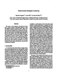
FIGURE 1.1 Left. two subspaces in 2D. Right. two 2D subspaces in 3D. The points in both 2D subspaces have been normalized to unit length. Due to noise, the points may not lie exactly on the subspace. One can observe that the angular distance finds the correct neighbors in most places except at the plane intersections. RD . The problem is illustrated in Figure 1.1, left, showing two linear subspaces and a number of outliers in R2 . A popular subspace clustering method [5][12][17] is based on spectral clustering, which relies on an affinity matrix that measures how likely any pair of points belong to the same subspace. Spectral clustering [15, 18] is a generic clustering method that groups a set of points into clusters based on their connectivity. The point connectivity is given as an N × N affinity matrix A with Aij close to 1 if point i is close to point j and close to zero if they are far away. The quality of the affinity matrix is very important for obtaining good clustering results. The affinity matrix for spectral subspace clustering will be described below. The spectral clustering algorithm proceeds by computing the matrix S = L−1/2 AL−1/2 , where L is a diagonal matrix with Lii as the sum of row i of A. It then computes the k-leading eigenvectors of S and obtains points in Rk from the eigenvectors. The points are then clustered by k-means or other clustering algorithm. The number k of clusters is assumed to be given. The spectral clustering algorithm is described in detail in Figure 1.2. Input: A set of points x1 , . . . , xN ∈ RD and the number k of clusters. 1. Construct the affinity matrix A ∈ RN ×N . PN 2. Construct the diagonal matrix L, with Lii = j=1 Aij . 3..Compute S = L−1/2 AL−1/2 . 4. Compute the matrix U = (u1 , . . . , uk ) ∈ Rn×k containing the leading k eigenvectors of S. 5. Treat each row of U as point in Rk and normalize them to unit length. 6. Cluster the n points of Rk into k clusters by k-means or other algorithm. 7. Assign the points xi to their corresponding clusters. FIGURE 1.2 The spectral clustering algorithm [15].

6


Affinity Matrix for Subspace Clustering. A common practice [5][12][17] before computing the affinity matrix is to normalize the points to unit length, as shown in Figure 1.1, right.. Then the following affinity measure based on the angle between the vectors has been proposed in [12] Aij = (

xTi xj )2α , kxi k2 kxj k2

(1.1)

where α is a tuning parameter, and the value α = 4 has been used in [12]. Fig 1.1, right shows two linear subspaces, where all points have been normalized. It is intuitive to find that the points tend to lie in the same subspace as their neighbors in angular distance except those near the intersection of the subspaces.

1.3

Scalable Subspace Clustering by Swendsen-Wang Cuts

This section presents a novel subspace clustering algorithm that formulates the subspace clustering problem as a MAP estimation of a posterior probability in a Bayesian framework and uses the Swendsen-Wang Cuts algorithm [2] for sampling and optimization. A subspace clustering solution can be represented as a partition (labeling) π : {1, ..., N } → {1, ..., M } of the input points x1 , . . . , xN ∈ RD . The number M ≤ N is the maximum number of allowed clusters. In this section is assumed that an affinity matrix A is given, representing the likelihood for any pair of points to belong to the same subspace. One form of A has been given in (1.1) and another one will be given in section 1.3.3.

1.3.1

Posterior Probability

A posterior probability will be used to evaluate the quality of any partition π. A good partition can then be obtained by maximizing the posterior probability in the space of all possible partitions. The posterior probability is defined in a Bayesian framework p(π) ∝ exp[−Edata (π) − Eprior (π)]. The normalizing constant is irrelevant in the optimization since it will cancel out in the acceptance probability. The data term Edata (π) is based on the fact that the subspaces are assumed to be linear. Given the current partition (labeling) π, for each label l an affine subspace Ll is fitted in a least squares sense through all points with label l. Denote the distance of a point x with label l to the linear space Ll as d(x, Ll ). Then the data term is M X X Edata (π) = d(xi , Ll ) (1.2) l=1 i,π(i)=l


7

The prior term Eprior (π) is set to encourage tightly connected points to stay in the same cluster. X Eprior (π) = −ρ log(1 − Aij ), (1.3) ∈E,π(i)6=π(j)

where ρ is a parameter controlling the strength of the prior term. It will be clear in the next section that this prior is exactly the Potts model (1.4) that would have Aij as the edge weights in the original SW algorithm.

1.3.2

Overview of the Swendsen-Wang Cuts Algorithm

The precursor of the Swenden-Wang Cuts algorithm is the Swendsen-Wang (SW) method [20], which is a Markov Chain Monte Carlo (MCMC) algorithm for sampling partitions (labelings) π : V → {1, ..., N } of a given graph G =< V, E >. The probability distribution over the space of partitions is the Ising/Potts model [16] X 1 βij δ(π(i) 6= π(j)]. (1.4) p(π) = exp[− Z ∈E

where βij > 0, ∀ < i, j >∈ E and N = |V |. The SW algorithm addresses the slow mixing problem of the Gibbs Sampler [10], which changes the label of a single node in one step. Instead, the SW algorithm constructs clusters of same label vertices in a random graph and flips together the label of all nodes in each cluster. The random graph is obtained by turning off (removing) all graph edges e ∈ E between nodes with different labels and removing each of the remaining edges < i, j >∈ E with probability e−βij . While the original SW method was developed originally for Ising and Potts models, the Swendsen-Wang Cuts (SWC) method [2] generalized SW to arbitrary posterior probabilities defined on graph partitions. The SWC method relies on a weighted adjacency graph G =< V, E > where each edge weight qe , e =< i, j >∈ E encodes an estimate of the probability that the two end nodes i, j belong to the same partition label. The idea of the SWC method is to construct a random graph in a similar manner to the SW but based on the edge weights, then select one connected component at random and accept a label flip of all nodes in that component with a probability that is based on the posterior probabilities of the before and after states and the graph edge weights. This algorithm was proved to simulate ergodic and reversible Markov chain jumps in the space of graph partitions and is applicable to arbitrary posterior probabilities or energy functions. From [2], there are different versions of the Swendsen-Wang Cut algorithm. The SWC-1 algorithm is used in this chapter, and is summarized in Figure 1.3. The set of edges C(V0 , Vl0 − V0 ), C(V0 , Vl − V0 ) from eq. (1.5) are the SW cuts defined in general as C(V1 , V2 ) = {< i, j >∈ E, i ∈ V1 , j ∈ V2 } The SWC algorithm could automatically decide the number of clusters,

8

Current Trends in Bayesian Methodology with Applications Input: Graph G =< V, E >, with weights qe , ∀e ∈ E, and posterior probability p(π|I). Initialize: A partition π : V → {1, ..., N } by random clustering for t = 1, . . . T , current state π, do 1. Find E(π) = {< i, j >∈ E, π(i) = π(j)} 2. For e ∈ E(π), turn µe = off with probability 1 − qe . 3. Vl = π −1 (l) is divided into Nl connected components Vl = Vl1 ∪ . . . ∪ Vlnl for l = 1, 2, . . . , N . 4. Collect all the connected components in set CP = {Vli : l = 1, . . . , N, i = 1, . . . , Nl }. 5. Select a connected component V0 ∈ CP with probability q(V0 |CP ) = 1 , say V0 ⊂ Vl . |CP | 6. Propose to assign V0 a new label cV0 = l0 with a probability q(l0 |V0 , π), thus obtaining a new state π 0 . 7. Accept the proposed label assignment with probability Y (1 − qe ) q(cV0 = l|V0 , π 0 ) p(π 0 |I) e∈C(V0 ,Vl0 −V0 ) 0 Y · · . (1.5) α(π → π ) = min(1, 0 (1 − qe ) q(cV0 = l |V0 , π) p(π|I) e∈C(V0 ,Vl −V0 ) end for Output: Samples π ∼ p(π|I).

FIGURE 1.3 The Swendsen-Wang Cut algorithm [2]. however in this chapter, as in most motion segmentation algorithms, it is assumed that the number of subspaces M is known. Thus the new label for the component V0 is sampled with uniform probability from the number M of subspaces: q(cV0 = l0 |V0 , π) = 1/M.

1.3.3

Graph Construction

Section 1.2 described a popular subspace clustering method based on spectral clustering. Spectral clustering optimizes an approximation of the normalized cut or the ratio cut [25], which are discriminative measures. In contrast, the proposed subspace clustering approach optimizes a generative model where the likelihood is based on the assumption that the subspaces are linear. It is possible that the discriminative measures are more flexible and work better when the linearity assumption is violated, and will be studied in future work. The following affinity measure, inspired by [12], will be used in this work θij Aij = exp(−m ¯ ), i 6= j (1.6) θ where θij is based on the angle between the vectors xi and xj , xTi xj θij = 1 − ( )2 , kxi k2 kxj k2 and θ¯ is the average of all θ. The parameter m is a tuning parameter to


9

control the size of the connected components obtained by the SWC algorithm. The subspace clustering performance with respect to this parameter will be evaluated in Section 1.4.2 for motion segmentation. The affinity measure based on the angular information between points enables to obtain the neighborhood graph, for example based on the k-nearest neighbors. After the graph has been obtained, the affinity measure is also used to obtain the edge weights for making the data driven clustering proposals in the SWC algorithm as well as for the prior term of the posterior probability. The graph G = (V, E) has as vertices the set of points that need to be clustered. The edges E are constructed based on the proposed distance measure from eq. (1.6). Since the distance measure is more accurate in finding the nearest neighbors (NN) from the same subspace, the graph is constructed as the k-nearest neighbor graph (kNN), where k is a given parameter. Examples of obtained graphs will be given in Section 1.4.2. Input: N points (x1 , . . . , xN ) from M subspaces Construct the adjacency graph G as a k-NN graph using eq (1.6). for r = 1, . . . , Q do Initialize the partition π as π(i) = 1, ∀i. for i = 1, . . . , N it do 1. Compute the temperature Ti using eq (1.7). 2. Run one step of the SWC algorithm 1.3 using p(π|I) = p1/Ti (π) in eq (1.5). end for Record the clustering result πr and the final probability pr = p(πr ). end for Output: Clustering result πr with the largest pr . FIGURE 1.4 The Swendsen-Wang Cuts algorithm for subspace clustering.

1.3.4

Optimization by Simulated Annealing

The SWC algorithm is designed for sampling the posterior probability p(π). To use SWC for optimization, a simulated annealing scheme should be applied while running the SWC algorithm. Simulated annealing means the probability used by the algorithm is not p(π) but p(π)1/T where T is a ”temperature” parameter that is large at the beginning of the optimization and is slowly decreased according to an annealing schedule. If the annealing scheduled is slow enough, it is theoretically guaranteed [11] that the global optimum of the probability p(π) will be found. In reality we use a faster annealing schedule, and the final partition π will only be a local optimum. We use an annealing schedule that is controlled by three parameters: the start temperature Tstart , the end temperature as Tend , and the number of iterations N it . The temperature at step i is calculated as

10

Current Trends in Bayesian Methodology with Applications Tend

Ti = log

, i = 1, N it

(1.7)

Tend Tend i N [e−exp( Tstart )]+exp( Tstart )

To better explore the probability space, we also use multiple runs with different random initializations. Then the final algorithm is shown in Figure 1.4.

1.3.5

Complexity Analysis

This section presents an evaluation of the computation complexity of the proposed SWC-based subspace clustering algorithm. To our knowledge, the complexity of SWC has not been calculated yet in the literature. Let N be the number of points in RD that need to be clustered. The computation complexity of the proposed subspace clustering method can be broken down as follows: • The adjacency graph construction is O(N 2 D log k) where D is the space dimension. This is because one needs to calculate the distance from each point to the other N − 1 points and use a heap to maintain its k-NNs. • Each of the N it iterations of the SWC algorithm involves: – Sampling the edges at each SWC step is O(|E|) = O(N ) since the k-NN graph G =< V, E > has at most 2kN edges. – Constructing connected components at each SWC step is O(|E|α(|E|)) = O(N α(N )) using the disjoint set forest data structure [9, 8]. The function α(N ) is the inverse of f (n) = A(n, n) where A(m, n) is the fast 1019729

growing Ackerman function [1] and α(N ) ≤ 5 for N ≤ 22 . – Computing Edata (π) involves fitting linear subspaces for each motion cluster, which is O(D2 N + D3 ) – Computing the Eprior (π) is O(N ). The number of iterations is N it = 2000, so all the SWC iterations take O(N α(N )) time. In conclusion, the entire algorithm complexity in terms of the number N of points is O(N 2 ) so it scales better than spectral clustering for large problems.

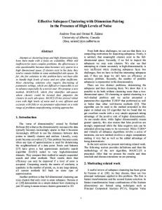
(a) 1RT2TC

(b) cars3

(c) articulated

FIGURE 1.5 Examples of SWC weighted graphs for a checkerboard (left), traffic (mid) and articulated (right) sequence. Shown are the feature point positions in the first frame. The edge intensities represent their weights from 0 (white) to 1 (black).


1.4

11

Application: Motion Segmentation

This section presents an application of the proposed subspace clustering algorithm to motion segmentation. Most recent works on motion segmentation use the affine camera model, which is approximatively satisfied when the objects are far from the camera. Under the affine camera model, a point on the image plane (x, y) is related to the real world 3D point X by x X =A , (1.8) y 1 where A ∈ R2×4 is the affine motion matrix. F T Let ti = (x1i , yi1 , x2i , yi2 , . . . , xF i , yi ) , i = 1, . . . .N be the trajectories of tracked feature points in F frames (2D images), where N is the number of trajectories. Let the measurement matrix W = [t1 , t2 , . . . , tN ] be constructed by assembling the trajectories as columns. If all trajectories undergo the same rigid motion, equation (1.8) implies that W can be decomposed into a motion matrix M ∈ R2F ×4 and a structure matrix S ∈ R4×N as W = MS  1  x1 x12 · · · x1N  1  1   y11 y21 · · · yN A    ..   .. . ..  X1 · · · XN . . . =  .  . . .   .  1 ··· 1  F F   xF x · · · x AF 1 2 N F y1F y2F · · · yN where Af is the affine object to world transformation matrix at frame f . It implies that rank(W ) ≤ 4. Since the entries of the last row of S are always 1, under the affine camera model, the trajectories of feature points from a rigidly moving object reside in an affine subspace of dimension at most 3. In general, we are given a measurement matrix W that contains trajectories from multiple possibly nonrigid motions. The task of motion segmentation is to cluster together all trajectories coming from each motion. A popular approach [5][12][17][24] is to project the trajectories to a lower dimensional space and to perform subspace clustering in that space, using spectral clustering as described in section 1.2. These methods differ in the projection dimension D and in the affinity measure A used for spectral clustering.

1.4.1

Dimension Reduction

Dimension reduction is an essential preprocessing step for obtaining a good motion segmentation. To realize this goal, the truncated SVD is often applied [5, 12, 17, 24].

12


To project the measurement matrix W ∈ R2F ×N to X = [x1 , ..., xN ] ∈ R , where D is the desired projection dimension, the matrix W is decomposed via SVD as W = U ΣV T and the first D columns of the matrix V are chosen as X T . The value of D for dimension reduction is also a major concern in motion segmentation. This value has a large impact on the speed and accuracy of the final result, so it is very important to select the best dimension to perform the segmentation. The dimension of a motion is not fixed, but can vary from sequence to sequence, and since it is hard to determine the actual dimension of the mixed space when multiple motions are present, different methods may have different dimensions for projection. The GPCA [24] suggests to project the trajectories onto a 5-dimensional space. ALC [17] chooses to use the sparsity-preserving dimension dsp = argmind≥2D log(2T /d) d for D-dimensional subspaces. The SSC [6] and LRR [13] simply projects the trajectories to the 4M subspace, where M is the number of motions. Some methods [5, 12] use an exhaustive search strategy to perform the segmentation in spaces with a range of possible dimensions and pick the best result. In this chapter, we find that projecting to dimension D = 2M + 1 can generate good results. The computation complexity of computing the SVD of a m × n matrix U when m >> n is O(mn2 + n3 ) [22]. If n >> m then it is faster to compute the SVD of U T , which takes O(nm2 + m3 ). Assuming that 2F