large software systems: efficient techniques tend to be too imprecise and often ..... If the call is virtual, the call node is connected to the entry node of each method ...
Scaling Regression Testing to Large Software Systems Alessandro Orso, Nanjuan Shi, and Mary Jean Harrold College of Computing Georgia Institute of Technology Atlanta, Georgia {orso|clarenan|harrold}@cc.gatech.edu
ABSTRACT When software is modified, during development and maintenance, it is regression tested to provide confidence that the changes did not introduce unexpected errors and that new features behave as expected. One important problem in regression testing is how to select a subset of test cases, from the test suite used for the original version of the software, when testing a modified version of the software. Regression-test-selection techniques address this problem. Safe regression-test-selection techniques select every test case in the test suite that may behave differently in the original and modified versions of the software. Among existing safe regression testing techniques, efficient techniques are often too imprecise and achieve little savings in testing effort, whereas precise techniques are too expensive when used on large systems. This paper presents a new regression-testselection technique for Java programs that is safe, precise, and yet scales to large systems. It also presents a tool that implements the technique and studies performed on a set of subjects ranging from 70 to over 500 KLOC. The studies show that our technique can efficiently reduce the regression testing effort and, thus, achieve considerable savings. Categories and Subject Descriptors: D.2.5 [Software Engineering]: Testing and Debugging—Testing tools; General Terms: Algorithms, Experimentation, Verification Keywords: Regression testing, testing, test selection, software evolution, software maintenance
1. INTRODUCTION As software evolves, regression testing is applied to modified versions of the software to provide confidence that the changed parts behave as intended and that the changes did not introduce unexpected faults, also known as regression faults. In the typical regression testing scenario, D is the developer of a software product P , whose latest version has been tested using a test suite T and then released. During maintenance, D modifies P to add new features and to fix faults. After performing the changes, D obtains a new ver-
Permission to make digital or hard copies of all or part of this work for personal or classroom use is granted without fee provided that copies are not made or distributed for profit or commercial advantage and that copies bear this notice and the full citation on the first page. To copy otherwise, to republish, to post on servers or to redistribute to lists, requires prior specific permission and/or a fee. SIGSOFT’04/FSE-12, Oct. 31–Nov. 6, 2004, Newport Beach, CA, USA. Copyright 2004 ACM 1-58113-855-5/04/0010 ...$5.00.
sion of the software product, P 0 , and needs to regression test it before committing the changes to a repository or before release. One important problem that D must face is how to select an appropriate subset T 0 of T to rerun on P 0 . This process is called regression test selection (RTS hereafter). A simple approach to RTS is to rerun all test cases in T on P 0 , that is, to select T 0 = T . However, rerunning all test cases in T can be expensive and, when there are limited changes between P and P 0 , may involve unnecessary effort. Therefore, RTS techniques (e.g., [2, 4, 6, 7, 9, 15, 17, 20, 22, 23]) use information about P , P 0 , and T to select a subset of T with which to test P 0 , thus reducing the testing effort. An important property for RTS techniques is safety. A safe RTS technique selects, under certain assumptions, every test case in the test suite that may behave differently in the original and modified versions of the software [17]. Safety is important for RTS techniques because it guarantees that T 0 will contain all test cases that may reveal regression faults in P 0 . In this paper, we are interested in safe RTS techniques only. Safe RTS techniques (e.g., [6, 7, 15, 17, 20, 22] differ in efficiency and precision. Efficiency and precision, for an RTS technique, are generally related to the level of granularity at which the technique operates [3]. Techniques that work at a high level of abstraction—for instance, by analyzing change and coverage information at the method or class level—are more efficient, but generally select more test cases (i.e., they are less precise) than their counterparts that operate at a fine-grained level of abstraction. Conversely, techniques that work at a fine-grained level of abstraction—for instance, by analyzing change and coverage information at the statement level—are precise, but often sacrifice efficiency. In general, for an RTS technique to be cost-effective, the cost of performing the selection plus the cost of rerunning the selected subset of test cases must be less than the overall cost of rerunning the complete test suite [23]. For regressiontesting cost models (e.g., [10, 11]), the meaning of the term cost depends on the specific scenario considered. For example, for a test suite that requires human intervention (e.g., to check the outcome of the test cases or to setup some machinery), the savings must account for the human effort that is saved. For another example, in a cooperative environment, in which developers run an automated regression test suite before committing their changes to a repository, reducing the number of test cases to rerun may result in early availability of updated code and improve the efficiency of the development process. Although empirical studies show that existing safe RTS techniques can be cost-effective [6, 7, 19],
such studies were performed using subjects of limited size. In our preliminary studies we found that, in many cases, existing safe techniques are not cost-effective when applied to large software systems: efficient techniques tend to be too imprecise and often achieve little or no savings in testing effort; precise techniques are generally too expensive to be used on large systems. For example, for one of the subjects studied, it took longer to perform RTS than to run the whole test suite. In this paper, we present a new RTS algorithm for Java programs that handles the object-oriented features of the language, is safe and precise, and still scales to large systems. The algorithm consists of two phases: partitioning and selection. The partitioning phase builds a high-level graph representation of programs P and P 0 and performs a quick analysis of the graphs. The goal of the analysis is to identify, based on information on changed classes and interfaces, the parts of P and P 0 to be further analyzed. The selection phase of the algorithm builds a more detailed graph representation of the identified parts of P and P 0 , analyzes the graphs to identify differences between the programs, and selects for rerun test cases in T that traverse the changes. Although the technique is defined for the Java language, it can be adapted to work with other object-oriented (and traditional procedural) languages. We also present DejaVOO: a tool that we developed and that implements our RTS technique. Finally, we present a set of empirical studies performed using DejaVOO on a set of Java subjects ranging from 70 to over 500 KLOC. The studies show that, for the subjects considered, our technique is considerably more efficient than an existing precise technique that operates at a fine-grained level of abstraction (89% on average for the largest subject). The studies also show that the selection achieves considerable savings in overall regression testing time. For the three subjects, our technique saved, on average, 19%, 36%, and 63% of the regression testing time. The main contributions of this paper are: • The definition of a new technique for RTS that is effective and can scale to large systems. • The description of a prototype tool, DejaVOO, that implements the technique. • A set of empirical studies that show and discuss the effectiveness and efficiency of our technique. These are the first studies that apply safe RTS to real systems of these sizes.
2. TWO-PHASE RTS TECHNIQUE The basic idea behind our technique is to combine the effectiveness of RTS techniques that are precise but may be inefficient on large systems (e.g., [7, 17, 18]) with the efficiency of techniques that work at a higher-level of abstraction and may, thus, be imprecise (e.g., [9, 22]). We do this using a two-phase approach that performs (1) an initial high-level analysis, which identifies parts of the system to be further analyzed, and (2) an in-depth analysis of the identified parts, which selects the test cases in T to rerun. We call these two phases partitioning and selection. In the partitioning phase, the technique analyzes the program to identify hierarchical, aggregation, and use relationships among classes and interfaces [13]. Then, the technique uses the information about these relationships, together with in-
formation about which classes and interfaces have syntactically changed, to identify the parts of the program that may be affected by the changes between P and P 0 . (Without loss of generality, we assume information about syntactically changed classes and interfaces to be available. This information can be easily gathered, for example, from configurationmanagement systems, IDEs that use versioning, or by comparison of the two versions of the program.) The output of this phase is a subset of the classes and interfaces in the program (hereafter, referred to as the partition). In the selection phase, the technique takes as input the partition identified by the first phase and performs edge-level test selection on the classes and interfaces in the partition. Edge-level test selection selects test cases by analyzing change and coverage information at the level of the flow of control between statements (see Section 2.2 for details). To perform edgelevel selection, we leverage an approach previously defined by some of the authors [7]. Because of the partitioning performed in the first phase, the low-level, expensive analysis is generally performed on only a small fraction of the whole program. Although only a part of the program is analyzed, the approach is still—under certain assumptions—safe because (1) the partitioning identifies all classes and interfaces whose behavior may change as a consequence of the modifications to P , and (2) the edgelevel technique we use on the selection phase is safe [7]. The assumptions for safety are discussed in Section 2.3. In the next two sections, we illustrate the two phases in detail, using the example provided in Figures 1 and 2. The example consists of a program P (Figure 1) and a modified version of P , P 0 (Figure 2). The differences between the two programs are highlighted in the figures. Note that, for ease of presentation, we align and use the same line numbering for corresponding lines of code in P and P 0 . Also for ease of presentation, in the rest of the paper we use the term type to indicate both classes and interfaces and the terms super-type and sub-type to refer to type-hierarchical relation (involving two classes, a class and an interface, or two interfaces).
2.1
Partitioning
The first phase of the approach performs a high-level analysis of P and P 0 to identify the parts of the program that may be affected by the changes to P . The analysis is based on purely syntactic changes between P and P 0 and on the relationships among classes and interfaces in the program.
2.1.1
Accounting for Syntactic Changes
Without loss of generality, we classify program changes into two groups: statement-level changes and declarationlevel changes. A statement-level change consists of the modification, addition, or deletion of an executable statement. These changes are easily handled by RTS: each test case that traverses the modified part of the code must be re-executed. Figures 1 and 2, at line 9, show an example of statementlevel change from P to P 0 . Any execution that exercises that statement, will behave differently for P and P 0 . A declaration-level change consists of the modification of a declaration. Examples of such changes are the modification of the type of a variable, the addition or removal of a method, the modification of an inheritance relationship, the change of type in a catch clause, or the change of a modifiers list (e.g., the addition of modifier “synchronized” to a method). These changes are more problematic for RTS than statement-level changes because they affect the behavior of
Program P 1: 2: 3: 4: 5: 6:
p u b l i c c l a s s SuperA { i n t i =0; public void foo ( ) { System . o u t . p r i n t l n ( i ) ; } }
7: p u b l i c c l a s s A e x t e n d s SuperA { 8: p u b l i c v o i d dummy ( ) { 9: i −−; 10: System . o u t . p r i n t l n (− i ) ; 11: }
12: } 13: public
c l a s s SubA e x t e n d s A { }
14: public class B { 15: p u b l i c void bar ( ) { 16: SuperA a=L i b C l a s s . getAnyA ( ) ; 17: a . foo ( ) ; 18: } 19: } 20: public
c l a s s SubB e x t e n d s B { }
21: public class C { 22: p u b l i c v o i d b a r (B b ) { 23: b . bar ( ) ; 24: } 25: }
Figure 1: Example program P . the program only indirectly, often in non-obvious ways. Figures 1 and 2 show an example of a declaration-level change: a new method f oo is added to class A, in P 0 (lines 12a–12c). In this case, the change indirectly affects the statement that calls a.f oo (line 17). Assume that LibClass is a class in the library and that LibClass.getAnyA() is a static method of such class that returns an instance of SuperA, A, or SubA. After the static call at line 16, the dynamic type of a can be SuperA, A, or SubA. Therefore, due to dynamic binding, the subsequent call to a.f oo can be bound to different methods in P and in P 0 : in P , a.f oo is always bound to SuperA.f oo, whereas in P 0 , a.f oo can be bound to A.f oo or SuperA.f oo, depending on the dynamic type of a. This difference in binding may cause test cases that traverse the statement at line 17 in P to behave differently in P 0 . Declaration-level changes have generally more complex effects than statement-level changes and, if not suitably handled, can cause an RTS technique to be imprecise, unsafe, or both. We will show how our technique suitably handles declaration-level changes in both phases.
2.1.2
Accounting for Relationships Between Classes
In this section, we use the example in Figures 1 and 2 to describe, intuitively, how our partitioning algorithm works and the rationale behind it. To this end, we illustrate different alternative approaches to partitioning, discuss their shortcomings, and motivate our approach. One straightforward approach for partitioning based on changes is to select just the changed types (classes or interfaces). Assume that the change at line 9 in Figures 1 and 2 is the only change between P and P 0 . In this case, any test case that behaves differently when run on P and P 0 must necessarily traverse statement 9 in P . Therefore, the straightforward approach, which selects only class A, would be safe and precise: in the second phase, the edge-level analysis of class A in P and P 0 would identify the change at statement 8 and select all and only test cases traversing it.
Program P ’ 1: 2: 3: 4: 5: 6:
p u b l i c c l a s s SuperA { i n t i =0; public void foo ( ) { System . o u t . p r i n t l n ( i ) ; } }
7: p u b l i c c l a s s A e x t e n d s SuperA { 8: p u b l i c v o i d dummy ( ) { 9: i ++; 10: System . o u t . p r i n t l n (− i ) ; 11: } 12 a : public void foo ( ) { 12 b : System . o u t . p r i n t l n ( i + 1 ) ; 12 c : } 12 d : } 13: public
c l a s s SubA e x t e n d s A { }
14: public class B { 15: p u b l i c void bar ( ) { 16: SuperA a=L i b C l a s s . getAnyA ( ) ; 17: a . foo ( ) ; 18: } 19: } 20: public
c l a s s SubB e x t e n d s B { }
21: public class C { 22: p u b l i c v o i d b a r (B b ) { 23: b . bar ( ) ; 24: } 25: }
Figure 2: Modified version of program P , P 0 . However, such a straightforward approach does not work in general for declaration-level changes. Assume now that the only change between P and P 0 is the addition of method f oo to A (12a–12c in P 0 ). As we discussed above, this change leads to a possibly different behavior for test cases that traverse statement 17 in P , which belongs to class B. Therefore, all such test cases must be included in T 0 , the set of test cases to rerun on P 0 . Conversely, any test case that does not execute that statement can be safely excluded from T 0 . Unfortunately, the straightforward approach would still select only class A. The edge-level analysis of A would then show that the change between A in P and A in P 0 is the addition of the overriding method A.f oo, a declaration-level change that does not affect directly any other statement in A. Therefore, the only way to select test cases that may be affected by the change would be to select all test cases that instantiate class A1 because these test cases may execute A.f oo in P 0 . Such an approach is clearly imprecise: some test cases may instantiate class A and never traverse a.f oo, but the approach would still select them. Moreover, this selection is also unsafe. If, in the second-phase, we analyze only class A, we will miss the fact that class SubA inherits from A. Without this information, we will not select test cases that traverse a.f oo when the dynamic type of a is SubA. Because these test cases may also behave differently in P and P 0 , not selecting them is unsafe. Because polymorphism and dynamic binding make RTS performed only on the changed types both unsafe and imprecise, a possible improvement is to select, when a type C has changed, the whole type hierarchy that involves C (i.e., all super- and sub-types of C. Considering our example, this strategy will select a partition that contains classes SuperA, A, and SubA. By analyzing SuperA, A, and SubA, the edge-level technique would (1) identify the inheritance 1 In this case, static calls are non-relevant because dynamic binding can occur only on actual instances.
algorithm buildIRG input: program P output: IRG G for P begin buildIRG 1: create empty IRG G 2: for each class and interface e ∈ P do 3: create node ne 4: GN = GN ∪ {ne } 5: end for 6: for each class and interface e ∈ P do 7: get direct super-type of e, s 8: GIE = GIE ∪ {hne , ns i} 9: for each type r ∈ P that e references do 10: GU E = GU E ∪ {hne , nr i} 11: end for 12: end for 13: return G end buildIRG
Figure 3: Algorithm for building an IRG. relationships correctly, (2) discover that a call to a.f oo may be bound to different methods in P and P 0 if the type of a is A or SubA, and (3) consequently select for rerun all test cases that instantiate A, SubA, or both. Thus, such a partitioning would lead to safe results. Although considering whole hierarchies solves the safety issue, the approach is still imprecise. Again, some test cases may instantiate class A or SubA and never invoke a.f oo. Such test cases behave identically in P and P 0 , but they would still be selected for rerun. To improve the precision of the selection, our partitioning technique considers, in addition to the whole hierarchy that involves a changed type, all types that explicitly reference types in the hierarchy. For our example, the partition would include SuperA, A, SubA, and B. By analyzing these four classes, an edge-level selection technique would be able to compute the hierarchy relationships, as discussed above, and also to identify the call site to a.f oo in B.bar as the point in the program where the program’s behavior may be affected by the change (details on how this is actually done are provided in Section 2.2). Therefore, the edge-level technique can select all and only the test cases that call a.f oo when the dynamic type of a is either A or SubA. This selection is safe and as precise as the most precise existing RTS techniques (e.g., [2, 7, 17]). It is important to note that no other type, besides the ones in the partition, must be analyzed by the edge-level technique. Because of the way the system is partitioned, any test case that behaves differently in P and P 0 must necessarily traverse one or more types in the partition, and would therefore be selected. Consider, for instance, class C of our example, which is not included in the partition. If a test case that exercises class C shows a different behavior in P and P 0 , it can only be because of the call to B.bar in C.bar. Therefore, the test case would be selected even if we consider only B. In summary, our partitioning technique selects, for each changed type (class or interface), (1) the type itself, (2) the hierarchy of the changed type, and (3) the types that explicitly reference any type in such hierarchy. Note that it may be possible to reduce the size of the partition identified by the algorithm by performing additional analysis (e.g., by distinguishing different kinds of use relationships among classes). However, doing so would increase the cost of the partitioning and, as the studies in Section 3 show, our current approach is effective in practice. In the next section, we present the algorithm that performs the selection.
SuperA
B
A
SubB
C
inheritance edge SubA
use edge
Figure 4: IRG for program P of Figure 1.
2.1.3
Partitioning Algorithm
Before describing the details of the partitioning algorithm, we introduce the program representation on which the algorithm operates: the interclass relation graph. The Interclass Relation Graph (IRG) for a program is a triple {N, IE, U E}: • N is the set of nodes, one for each type. • IE ⊂ N × N is the set of inheritance edges. An inheritance edge between a node for type e1 and a node for type e2 indicates that e1 is a direct sub-type of e2 . • U E ⊂ N ×N is the set of use edges. A use edge between a node for type e1 and a node for type e2 indicates that e1 contains an explicit reference to e2 .2 Figure 3 shows the algorithm for building an IRG, buildIRG. For simplicity, in defining the algorithms, we use the following syntax: ne indicates the node for a type e (class or interface); GN , GIE , and GU E indicate the set of nodes N , inheritance edges IE, and use edges U E for a graph G, respectively. Algorithm buildIRG first creates a node for each type in the program (lines 2–5). Then, for each type e, the algorithm (1) connects ne to the node of its direct super-type through an inheritance edge (lines 7–8), and (2) creates a use edge from each nd to ne , such that d contains a reference to e (lines 9–11). Figure 4 shows the IRG for program P in Figure 1. The IRG represents the six classes in P and their inheritance and use relationships. Figures 5, 6, and 7 show our partition algorithm, computePartition. The algorithm inputs the set of syntacticallychanged types C and two IRGs, one for the original version of the program and one for the modified version of the program. As we mentioned above, change information can be easily computed automatically. First, algorithm computePartition adds to partition P art all hierarchies that involve changed types. For each type e in the changed-type set C, the algorithm adds to P art e itself (line 3) and all sub- and super-types of e, by calling procedures addSubTypes and addSuperTypes (lines 4 and 5). If s, the super-type of e in P , and s0 , the super-type of e in P 0 , differ (lines 6–8), the algorithm also adds all super-types of s0 to the partition (line 9). This operation is performed to account for cases in which type e is moved to another inheritance hierarchy. In these cases, changes to e may affect not only types in e’s old hierarchy, but also types in e’s new hierarchy. Consider our example program in Figure 1 and its corresponding IRG in Figure 4. Because the only changed type is class A, at this point in the algorithm P art would contain classes A, SubA, and SuperA. 2 The fact that e1 contains an explicit reference to e2 means that e1 uses e2 (e.g., by using e2 in a cast operation, by invoking one of e2 ’s methods, by referencing one of e2 ’s field, or by using e2 as an argument to instanceof).
algorithm computePartition input: set of changed types C, IRG for P , G IRG for P 0 , G0 declare: set of types T mp, initially empty output: set of types in the partition, P art begin computePartition 1: P art = ∅ 2: for each type e ∈ C do 3: P art = P art ∪ {e} 4: P art = P art ∪ addSubTypes(G, e) 5: P art = P art ∪ addSuperTypes(G, e) 6: ns = n ∈ G, hne , ni ∈ GIE 7: ns0 = n ∈ G0 , hne , ni ∈ G0IE 8: if s 6= s0 then 9: P art = P art ∪ {s0 } 10: P art = P art ∪ addSuperTypes(G0 , s0 ) 11: end if 12: end for 13: for each type p ∈ P art do 14: for each edge v = hnd , np i ∈ GU E do 15: T mp = T mp ∪ {d} 16: end for 17: end for 18: P art = P art ∪ T mp 19: return P art end computePartition
procedure addSubTypes input: IRG G, type e output: set of all sub-types of e, S begin addSubTypes 19: S = ∅ 20: for each node ns ∈ G, hns , ne i ∈ GIE do 21: S = S ∪ {s} 22: S = S ∪ addSubTypes(G, s) 23: end for 24: return S end addSubTypes
Figure 6: Procedure addSubTypes. procedure addSuperTypes input: IRG G, type e output: set of all super-types of e, S begin addSuperTypes 25: S = ∅ 26: while ∃ns ∈ G, hne , ns i ∈ GIE do 27: S = S ∪ {s} 28: e = s 29: end while 30: return S end addSuperTypes
Figure 5: Algorithm computePartition.
Figure 7: Procedure addSuperTypes.
Second, for each type p currently in the partition, computePartition adds to a temporary set T mp all types that reference p directly (lines 13–17). In our example, this part of the algorithm would add class B to T . Finally, the algorithm adds the types in T mp to P art and returns P art. Procedure addSubTypes inputs an IRG G and a type e, and returns the set of all types that are sub-types of e. The procedure performs, through recursion, a backward traversal of all inheritance edges whose target is node ne . Procedure addSuperTypes also inputs an IRG G and a type e, and returns the set of all types that are super-types of e. The procedure identifies super-types through reachability over inheritance edges, starting from e.
following we provide an overview of this part of the technique. Reference [7] provides additional details.
Complexity. Algorithm buildIRG makes a single pass over each type t, to identify t’s direct super-class and classes referenced by t. Therefore, the worst-case time complexity of the algorithm is O(m), where m is the size of program P . Algorithm computePartition performs reachability from each changed type. The worst case time complexity of the algorithm is, thus, |C|O(n2 ), where C is the set of changed types and n is the number of nodes in the IRG for P (i.e., the number of classes and interfaces in the program). However, this complexity corresponds to the degenerate case of programs with n types and an inheritance tree of depth O(n). In practice, the depth of the inheritance tree can be approximated with a constant, and the overall complexity of the partitioning is linear in the size of the program. In fact, our experimental results show that our partition algorithm is very efficient in practice; for the largest of our subjects, JBoss, which contains over 2,400 classes and over 500 KLOC, our partitioning process took less than 15 seconds to complete.
2.2 Selection The second phase of the technique (1) computes change information by analyzing the types in the partition identified by the first phase, and (2) performs test selection by matching the computed change information with coverage information. To perform edge-level selection, we use an approach previously defined by some of the authors [7]. In the
2.2.1
Computing Change Information
To compute change information, our technique first constructs two graphs, G and G0 , that represent the parts of P and P 0 in the partition identified by the partitioning phase. To adequately handle all Java language constructs, we defined a new representation: the Java Interclass Graph. A Java Interclass Graph (JIG) extends a traditional control flow graph, in which nodes represent program statements and edges represent the flow of control between statements. The extensions account for various aspects of the Java language, such as inheritance, dynamic binding, exception handling, and synchronization. For example, all occurrences of class and interface names in the graph are fully qualified, which accounts for possible changes of behavior due to changes in the type hierarchy. The extensions also allow for safely analyzing subsystems if the part of the system that is not analyzed is unchanged (and unaffected by the changes), as described in detail in Reference [7]. For the sake of space, instead of discussing the JIG in detail, we illustrate how we model dynamic binding in the JIG using our example programs P and P 0 (see Figures 1 and 2). The top part of Figure 8 shows two partial JIGs, G and G0 , that represent method B.bar in P and P 0 . In the graph, each call site (lines 16 and 17) is expanded into a call and a return node (nodes 16a and 16b, and 17a and 17b). Call and return nodes are connected by a path edge (edges (16a,16b) and (17a,17b)), which represents the path through the called method. Call nodes are connected to the entry node(s) of the called method(s) with a call edge. If the call is static (i.e., not virtual), such as the call to LibClass.getAnyA(), the call node has only one outgoing call edge, labeled call. If the call is virtual, the call node is connected to the entry node of each method that can be bound to the call. Each call edge from the call node to the entry node of a method m is labeled with the type of the receiver instance that causes m to be bound to the call. In the example considered, the call to a.f oo at node 17a is a virtual call. In P , although a can have dynamic type SuperA, A, or SubA, the call is
�
�
E
�
�
�
�
�
�
�
� F
G
H
�
�
I
�
�
J
�
�
�
�
E
�
� �
�
�
�
�
�
�
�
�
H
�
G
H
�
�
�
� �
F
I
�
�
J
�
�
�
�
�
H
�
�
�
H
H
K K
�
�
�
�
�
�
�
�
�
�
�
�
� �
�
�
�
�
�
�
�
�
�
�
� �
�
�
�
� �
�
�
�
�
�
�
�
�
�
�
�
�
�
�
�
�
�
�
� �
�
�
�
�
� �
�
�
�
�
the end of the synchronous walk, the set of dangerous edges for P consists of edges (17a,3,“SubA”) and (17a,3, “A”). In the next section, we describe how dangerous edges are matched with coverage information to select for rerun all test cases in T that traverse edge (17a,3,“SubA”) or edge (17a,3,“A”), that is, all test cases that execute the call at statement 17 with a’s dynamic type being A or SubA.
�
�
�
2.2.2
�
�
�
�
�
�
�
�
�
�
�
�
�
�
�
�
�
�
�
�
�
Performing Test Selection
�
�
?
B
C
�
�
�
�
@ >
A
�
�
�
>
1 �
=
D
�
,
,
-
-
.
;
0
�
�