While its quadratic programming formulation has the important computational .... Inspired by the MEB algorithms and the use of core-sets, we propose in this ...
Scaling up Support Vector Data Description by Using Core-Sets Calvin S. Chu
Ivor W. Tsang
James T. Kwok
Department of Computer Science Hong Kong University of Science and Technology Clear Water Bay Hong Kong E-mail: {cscalvin,ivor,jamesk}@cs.ust.hk
Abstract— Support vector data description (SVDD) is a powerful kernel method that has been commonly used for novelty detection. While its quadratic programming formulation has the important computational advantage of avoiding the problem of local minimum, this has a runtime complexity of O(N 3 ), where N is the number of training patterns. It thus becomes prohibitive when the data set is large. Inspired from the use of core-sets in approximating the minimum enclosing ball problem in computational geometry, we propose in this paper an approximation method that allows SVDD to scale better to larger data sets. Most importantly, the proposed method has a running time that is only linear in N . Experimental results on two large real-world data sets demonstrate that the proposed method can handle data sets that are much larger than those that can be handled by standard SVDD packages, while its approximate solution still attains equally good, or sometimes even better, novelty detection performance.
I. I NTRODUCTION In recent years, there has been a lot of interest on using kernels in various aspects of machine learning, such as classification, regression, clustering, ranking and principal component analysis [1], [2], [3]. A well-known example in supervised learning is the support vector machines (SVMs). The basic idea of kernel methods is to map the data from an input space to a feature space F via some map ϕ, and then apply a linear procedure there. It is now well-known that the computations do not involve ϕ explicitly, but depend only on the inner product defined in F, which in turn can be obtained efficiently from a suitable kernel function (the “kernel trick”). In this paper, we will focus on the use of kernel methods in novelty detection, in which one aims at differentiating known objects (or normal patterns) from unknown objects (or outliers) [4], [5], [6]. There are a large number of realworld novelty detection applications, such as the detection of unusual vibration signatures in jet engines [7] or the detection of new events from newswire stories in text mining [8]. As only the positive information is available, novelty detection is more challenging than supervised learning. Traditionally, novel patterns are detected by either estimating the density function of the normal patterns, or by finding a small set Q such that P (x ∈ Q) = α for some fixed α ∈ (0, 1] (quantile estimation). However, both depend critically on the parametric form of the density function, and can fail miserably when the parametric form is incorrect.
Instead of estimating the density or quantile, a simpler task is to model the support of the data distribution directly. Tax and Duin proposed the support vector data description (SVDD) [9], which uses a ball with minimum volume to enclose most of the data. Computationally, this leads to a quadratic programming (QP) problem, which has the important advantage that the solution obtained is always globally optimal. Moreover, as with other kernel methods, SVDD works well with highdimensional data and can be easily kernelized by replacing the dot product between patterns with the corresponding kernel evaluation. Besides using a ball, one can also use a hyperplane. Sch¨olkopf et al. proposed the one-class SVM that separates the normal patterns from the outliers (represented by the origin) with maximum margin [10], [11]. Again, computationally, this leads to a QP problem. Moreover, when Gaussian kernels are used, the one-class SVM solution is equivalent to that of the SVDD. Recently, Lanckriet et al. proposed the single-class minimax probability machine (MPM) [12] that is also based on the use of hyperplanes. A distinctive aspect of the single-class MPM is that it can provide a distribution-free probability bound. Specifically, given only the mean and covariance matrix of a distribution and without making any other distributional assumption, it seeks the smallest half-space Q(w, b) = {z | w′ z ≥ b}, not containing the origin, that minimizes the worst-case probability of a data point falling outside of Q. However, despite its interesting theoretical properties, the single-class MPM has high false negative rate in practice [13], and some uncertainty information on the covariance matrix is required to alleviate this problem. While the QP formulations in both SVDD and one-class SVM have the computational advantage of avoiding the problem of local minimum, their runtime complexities are of O(N 3 ), where N is the number of training patterns. In order to allow the QP to scale better to larger data sets, Sch¨olkopf et al. [11] suggested the use of a modified version of the sequential minimal optimization (SMO) algorithm [14]. However, as will be demonstrated experimentally in Section IV, a SMObased implementation of the one-class SVM can still suffer from scale-up problems. A more radical possibility to improve the scale-up behavior
is by changing the formulation altogether, such as from quadratic programming to linear programming (LP) [15]. In general, LPs can handle large data sets, especially with the use of column generation algorithms. However, the LP formulation in [15] is based on minimizing the mean value of the outputs on the normal patterns, which is less intuitive than minimizing the size of the ball as in SVDD or maximizing the margin as in one-class SVM. Viewing from a broader perspective, the ball-finding problem in SVDD is related to the minimum enclosing ball (MEB) problem in computational geometry [16], [17], [18]. Given a set S of points, the MEB of S, denoted by MEB(S), is the unique minimum radius ball that contains all of S. Recently, Badoiu et al. [16] showed that there exist efficient algorithms for finding its (1 + ǫ)-approximation1 . The main idea is to use only a small subset of points, called the core-set2 , in computing the approximate solution. The resultant core-set can be shown to be of size O(1/ǫ). Subsequently, the algorithm has a running time that is only linear in the number of points, and is thus readily scalable. However, despite the apparent similarity between the MEB problem and SVDD, these MEB algorithms cannot be readily applied to SVDD. A crucial distinction is that the MEB is required to enclose all data points in S, including even outliers. SVDD, on the other hand, allows outliers to remain outside the ball with the use of slack variables. Moreover, most existing algorithms for finding the MEB can only handle low-dimensional data, whereas SVDD has to operate in the possibly infinite-dimensional kernel-induced feature space. Inspired by the MEB algorithms and the use of core-sets, we propose in this paper a procedure for speeding up SVDD. Most importantly, we will show that its running time is only linear in the number of training patterns (N ), instead of the O(N 3 ) complexity for standard SVDD. The rest of this paper is organized as follows. Section II first introduces SVDD. Section III then describes our proposed speed-up procedure. Experimental results on two large, real-world data sets are presented in Section IV, and the last section gives some concluding remarks. II. S UPPORT V ECTOR DATA D ESCRIPTION Given a set S = {x1 , . . . , xN }, SVDD attempts to find a small ball, with center c and radius R, that contains most of the patterns in S. To allow for the presence of outliers, slack variables ξi ’s are introduced as in other kernel methods. The (primal) optimization problem is then
Here, ν ∈ (0, 1) is a user-provided parameter specifying an upper bound on the fraction of outliers. The corresponding dual problem is: maxαi
N X i=1
s.t.
αi x′i xi −
N X
αi αj x′i xj
i,j=1
1 , i = 1, . . . , N, 0 ≤ αi ≤ νN N X αi = 1. i=1
This is a quadratic programming problem in the N variables α1 , . . . , αN . As mentioned in Section I, its solution is guaranteed to be globally optimal. By using the Karush-Kuhn-Tucker (KKT) PNcondition, the center can be obtained from the αi ’s as c = i=1 αi xi . Moreover, the radius R can also be computed by calculating the distance between c and any support vector xi on the boundary of the ball. On testing, a new pattern z will be predicted to be an outlier if its distance from the center c is larger than the radius; otherwise, it will be predicted as normal. Finally, notice that SVDD can be easily kernelized by simply replacing x′i xj in the computations by k(xi , xj ), where k(·, ·) is some suitable kernel function. III. S CALING UP SVDD In this Section, we borrow the idea of core-sets in the MEB algorithms to scale up SVDD. The basic procedure is as follows. First, we construct an initial core-set containing only one normal pattern (Section III-A), and patterns are then added to it incrementally. Instead of using all N training patterns in SVDD’s QP, we only use patterns in this core-set to form the QP (Section III-B). By keeping the size of the core-set small (say, of size n 1, such that R1 is a small number. Moreover, note that R1 ≥ RM EB(S) /k.
(1)
B. Iterative Procedure After initialization, patterns will be added to the coreset incrementally. In the following, we denote the center, radius and the core-set at the ith iteration by ci , Ri and Si respectively. Moreover, as in traditional SVDD, we assume that the user will supply the value of ν, which is an upper bound on the fraction of outliers. The following iterative procedure is then taken: 1) Initialize R1 and z as mentioned in Section III-A. Set S1 = {z}, c1 = z and i = 1. 2) Find the set Pi of patterns in S that fall outside the (1 + ǫ)-ball Bci ,(1+ǫ)Ri . In other words, Pi = {x ∈ S | kx − ci k > (1 + ǫ)Ri }. 3) If the size of Pi is smaller than νN , the expected number of outliers, then terminate. 4) Otherwise, expand the core-set by including the pattern in Pi \ Si that is closest to ci . Denote the expanded core-set by Si+1 . 5) Run SVDD on Si+1 , and obtain the new center ci+1 and radius Ri+1 . 6) Enforce the constraint that Ri+1 ≥ (1 + δǫ)Ri ,
(2)
where δ is a small, user-defined constant. In other words, the radius must increase by at least δǫRi at the ith iteration. As will be discussed in section III-C, this constraint is crucial for bounding the time complexity. 7) Increment i by 1 and go back to Step 2.
this Section, we will still be able to show that the algorithm in Section III-B has a time complexity that is only linear in the number of training patterns N . Consider first the initialization step. As n0 is fixed, both running the initial SVDD and the finding of z only take O(1) time. In determining the initial radius R1 , the finding of y takes O(N ) time. So, the total time required for initialization is O(N ). At the ith iteration, Ri is increased by at least δǫ )RM EB(S) , k on using (1) and (2). Obviously, RM EB(S) is an upper bound on the radius of the ball required. Therefore, the total number k of iterations is no more than δǫ = O(1/ǫ). At each iteration, one pattern will be added to the coreset in step 4. Hence, the size of Si is i and consequently ci is a linear combination of i ϕ-mapped patterns. Thus, at the ith iteration, step 4 requires takes O(iN ) time, while running SVDD in step 5 takes O((i + 1)3 ) = O(i3 ) time. The other steps take only constant time. And so the total time for the ith iteration is O(iN + i3 ). The total time for the whole procedure, including initialization and M = O(1/ǫ) iterations, is then: δǫRi > δǫRi−1 > · · · > δǫR1 ≥ (
T
= O(N ) + = O(N ) +
M X
O(iN + i3 )
i=1 M X i=1
!
i O(N ) +
= O(M 2 N + M 4 ) 1 1 = O( 2 N + 4 ). ǫ ǫ
M X
i3
i=1
(3)
For a fixed ǫ, T is thus linear in N , instead of O(N 3 ) in traditional SVDD. IV. E XPERIMENT In this Section, we perform experiments on two real-world datasets, the BioID Face Database3 (Section IV-A) and the MNIST handwritten digits database4 (Section IV-B). In the sequel, we denote the proposed method by CSVDD, which stands for “Core-set Support Vector Data Description”. It will be compared with two standard SVDD packages: the data description toolbox (dd tools) and the SMO-based LIBSVM5 [19]. All these are implemented in MATLAB, with MOSEK6 (version 3) being used as the underlying QP solver in both dd tools and CSVDD. Experiments are run on a P4-2.24GHz machine, with 1G RAM, running Windows XP. Moreover, in
C. Time Complexity In the MEB problem, it can be shown that the number of iterations in a similar procedure as above is of O(1/ǫ2 ) [16] (or even O(1/ǫ) when the furthest pattern is used in each iteration [17]). However, as mentioned in Section I, these results cannot be directly applied here because of the presence of slack variables in the SVDD formulation. Nevertheless, in
3 The BioID Face Database can be downloaded from http://www.humanscan.de/support/downloads/facedb.php. 4 The MNIST database can be downloaded from ftp://ftp.kyb.tuebingen.mpg.de/pub/bs/data. 5 dd tools and LIBSVM can be downloaded from http://www.ph.tn.tudelft.nl/∼davidt/dd toolbox.html and http://www.csie.ntu.edu.tw/∼cjlin/libsvm respectively. 6 MOSEK can be downloaded from http://www.mosek.com.
all the experiments, we set n0 in the initialization step to 20, k in (1) to 10, and δ in (2) to 0.01ǫ. Several criteria are used to compare the novelty detectors. The first set of criteria, namely the AUC error, FP and FN, are based on the ROC (receiver operating characteristic) graph [20], which plots the true positive (TP) rate on the Y -axis and the false positive (FP) rate on the X-axis. TP and FP are defined by TP FP
= =
(a) Images cropped from the database.
positives correctly classified , total positives negatives incorrectly classified , total negatives
(b) Images generated by tensor voting.
respectively. Here, outliers are treated as positives while normal patterns as negatives. Similarly, the false negative rate (FN) is defined as FN =
positives incorrectly classified . total positives
AUC stands for the area under the ROC curve, and the AUC error is defined as (1 − AUC). The AUC error is always between 0 and 1. A perfect novelty detector will have zero AUC error, while random guessing will have an AUC error of 0.5. The second criterion is the CPU time (in seconds) required by Matlab for the whole procedure. To reduce statistical variability, results here are based on averages over 20 random repetitions.
(c) Non-face images.
Fig. 1.
TABLE I R ESULTS ON THE FACE DATA SET ( NUMBERS IN BRACKETS ARE THE STANDARD DEVIATIONS ).
size of tr set 100
300
A. Face Database This database contains 1,521 gray level images, each showing the frontal view of a face of one out of 23 different test persons. Because the images are taken under a large variety of background, the faces need to be first manually aligned and cropped, producing images with a resultant size of 25 × 25. Moreover, in order to better evaluate the scale-up capabilities, we use tensor voting [21] to expand this database to a total of 75,787 face images, with grey scale from 0 to 255. No preprocessing, such as illumination correction, mean value normalization and histogram equalization are performed. Moreover, to provide outliers in the experiments, we gather some non-face images from images of natural scenes, buildings and textures. Sample images are shown in Figure 1. During training, we use 100 to 30,000 face images sampled from the 75,787 images generated above, and no non-face image is used. The test set consists of 2,000 face and 2,000 non-face images. We use the Gaussian kernel � � kx − yk2 k(x, y) = exp − , (4) 2σ 2 with σ = 500. Moreover, ν is always set to 0.05. Table I compares CSVDD (with ǫ = 0.3) with the standard SVDD packages of dd tools and LIBSVM. As can be seen, the AUC errors of all three are comparable for this value of ǫ, and CSVDD has a lower FN but higher FP. Thus, although CSVDD is only an approximate solution, results here indicated that its solution is still close to optimal.
Sample images used in the experiment in Section IV-A.
600
1000
3000
6000 10000 20000 30000
method dd tools LIBSVM CSVDD dd tools LIBSVM CSVDD dd tools LIBSVM CSVDD dd tools LIBSVM CSVDD dd tools LIBSVM CSVDD CSVDD CSVDD CSVDD CSVDD
AUC error 0.0489 (0.003) 0.0489 (0.003) 0.0484 (0.004) 0.0499 (0.004) 0.0499 (0.004) 0.0507 (0.007) 0.0488 (0.003) 0.0488 (0.003) 0.0504 (0.005) 0.0492 (0.002) 0.0492 (0.002) 0.0468 (0.005) 0.0497 (0.001) 0.0497 (0.001) 0.0478 (0.005) 0.0531 (0.006) 0.0499 (0.004) 0.0492 (0.005) 0.0498 (0.005)
FN 0.28 (0.04) 0.28 (0.04) 0.02 (0.02) 0.14 (0.01) 0.14 (0.01) 0.01 (0.01) 0.10 (0.01) 0.10 (0.01) 0.02 (0.01) 0.08 (0.00) 0.08 (0.00) 0.01 (0.01) 0.06 (0.01) 0.06 (0.01) 0.01 (0.01) 0.01 (0.01) 0.02 (0.01) 0.01 (0.01) 0.02 (0.01)
FP 0.07 (0.01) 0.07 (0.01) 0.28 (0.19) 0.09 (0.01) 0.09 (0.01) 0.30 (0.18) 0.11 (0.01) 0.11 (0.01) 0.24 (0.06) 0.12 (0.01) 0.12 (0.01) 0.27 (0.09) 0.14 (0.01) 0.14 (0.01) 0.23 (0.06) 0.25 (0.06) 0.21 (0.05) 0.26 (0.08) 0.23 (0.07)
Figure 2 compares their speeds. When the training set is small, both dd tools and LIBSVM are faster than CSVDD. This, nevertheless, is not surprising as CSVDD has to run the QP multiple times. In fact, under this situation, there is no scale-up problem and the standard SVDD packages should be the preferred choice. The real power of CSVDD, however, can be seen as the training set gets larger. This can be seen more clearly in Figure 2, which shows that CSVDD then becomes significantly faster than the other two traditional SVDD approaches. With 6,000 or more training patterns, both dd tools and LIBSVM cannot be run on the machine used in the experiment. We then vary the value of ǫ used in CSVDD. Table II shows that there is only very small difference in terms of novelty
3
10
CSVDD (ε=0.15) CSVDD (ε=0.2) CSVDD (ε=0.3) CSVDD (ε=0.4) CSVDD (ε=0.5)
120
100 size of core−set
CPU time (in second, log scale)
140
CSVDD (ε=0.15) CSVDD (ε=0.2) CSVDD (ε=0.3) CSVDD (ε=0.4) CSVDD (ε=0.5) SVDD LIBSVM
4
10
2
10
1
10
80
60
40
0
10
20 −1
10
2
3
10
Fig. 2.
4
10 10 size of training set (in log scale)
5
2
10
CPU time vs number of training patterns (Face database).
detection performance when ǫ is changed in the range tested. However, as can be seen in (3), a smaller value of ǫ leads to longer training time (Figure 2). Figure 3 plots the size of the resultant core-set, which is the same as the number of iterations, with the value of ǫ. As expected, the resultant coreset is only a very small subset of the training set, and its size also grows slowly with increasing training set size. Moreover, as discussed in Section III-C, the number of iterations is of O(1/ǫ), and this rising trend with 1/ǫ can also be clearly observed.
10
Fig. 3.
3
4
10 10 size of training set (in log scale)
5
10
Size of the core-set at different values of ǫ (Face database).
ν is set to 0.9. On this database, the LIBSVM package cannot converge to the correct solution, and so only dd tools and CSVDD can be compared.
(a) Digit 1 images.
TABLE II CSVDD R ESULTS AT DIFFERENT VALUES OF ǫ (FACE DATABASE ).
ǫ 0.5
0.4
size of tr set 100 300 600 1000 3000 6000 10000 20000 30000 100 300 600 1000 3000 6000 10000 20000 30000
AUC error 0.0526 (0.007) 0.0496 (0.007) 0.0518 (0.006) 0.0492 (0.009) 0.0535 (0.006) 0.0510 (0.006) 0.0488(0.008) 0.0527 (0.008) 0.0496 (0.005) 0.0528 (0.007) 0.0510 (0.007) 0.0514 (0.007) 0.0476 (0.005) 0.0510 (0.005) 0.0509 (0.005) 0.0539 (0.007) 0.0502 (0.008) 0.0518 (0.006)
ǫ 0.2
0.15
size of tr set 100 300 600 1000 3000 6000 10000 20000 30000 100 300 600 1000 3000 6000 10000 20000 30000
AUC error 0.0484 (0.004) 0.0490 (0.006) 0.0524 (0.006) 0.0492 (0.005) 0.0503 (0.006) 0.0490 (0.004) 0.0484 (0.005) 0.0482 (0.004) 0.0477 (0.006) 0.0496 (0.004) 0.0482 (0.004) 0.0495 (0.004) 0.0472 (0.005) 0.0483 (0.003) 0.0490 (0.005) 0.0483 (0.003) 0.0488 (0.005) 0.0460 (0.004)
B. MNIST Database The second set of experiments is performed on the MNIST database, which contains 20×20 grey-level images of the digits 0, 1, . . . , 9. In this experiment, we treat the digit one images as normal patterns and all others as outliers. Sample images are shown in Figure 4. A total of 6,742 digit one images are used to form the training set, while the test set has 10,000 images, with 1,135 of them belonging to the digit one. Again, we use the same Gaussian kernel in (4), with σ = 8, and also
(b) Outlier images.
Fig. 4.
Sample images used in the experiment in Section IV-B.
Table III compares the novelty detection performance. It can be seen that CSVDD is even more accurate than dd tools in terms of AUC error. Variations of the CPU time and size of the core-set with the number of training patterns are shown in Figures 5 and 6 respectively. Again, standard SVDD is faster than CSVDD when the data set is small. However, CSVDD becomes significantly faster on large data sets. With 3,000 or more training patterns, dd tools cannot be run on the machine used in the experiment. Finally, other trends as discussed in Section IV-A can also be observed here. V. C ONCLUSION In this paper, we proposed a scale-up algorithm for SVDD based on the idea of core-sets in computational geometry. Unlike the standard SVDD which has a runtime complexity of O(N 3 ), where N is the number of training patterns, the proposed procedure has a running time which is only linear in N . Experimental results show that this allows SVDD to be
TABLE III R ESULTS ON THE MNIST DATA SET (N UMBERS IN BRACKETS ARE THE STANDARD DEVIATIONS ).
size of tr set 100
300
600
1000
2000
3000
6000
method dd tools CSVDD (ǫ = 0.3) CSVDD (ǫ = 0.4) CSVDD (ǫ = 0.5) dd tools CSVDD (ǫ = 0.3) CSVDD (ǫ = 0.4) CSVDD (ǫ = 0.5) dd tools CSVDD (ǫ = 0.3) CSVDD (ǫ = 0.4) CSVDD (ǫ = 0.5) dd tools CSVDD (ǫ = 0.3) CSVDD (ǫ = 0.4) CSVDD (ǫ = 0.5) dd tools CSVDD (ǫ = 0.3) CSVDD (ǫ = 0.4) CSVDD (ǫ = 0.5) CSVDD (ǫ = 0.3) CSVDD (ǫ = 0.4) CSVDD (ǫ = 0.5) CSVDD (ǫ = 0.3) CSVDD (ǫ = 0.4) CSVDD (ǫ = 0.5)
AUC error 0.145 (0.057) 0.033 (0.038) 0.039 (0.074) 0.035 (0.035) 0.162 (0.040) 0.036 (0.041) 0.054 (0.110) 0.078 (0.148) 0.159 (0.030) 0.126 (0.148) 0.176 (0.219) 0.175 (0.218) 0.161 (0.020) 0.084 (0.114) 0.097 (0.145) 0.119 (0.175) 0.162 (0.020) 0.053 (0.078) 0.063 (0.096) 0.086 (0.139) 0.067 (0.104) 0.091 (0.144) 0.090 (0.131) 0.067 (0.091) 0.091 (0.140) 0.106 (0.170)
FN 0.20 (0.12) 0.15 (0.15) 0.16 (0.17) 0.15 (0.17) 0.13 (0.09) 0.09 (0.10) 0.11 (0.12) 0.14 (0.13) 0.09 (0.06) 0.09 (0.10) 0.19 (0.23) 0.13 (0.18) 0.10 (0.05) 0.10 (0.11) 0.12 (0.15) 0.12 (0.13) 0.08 (0.04) 0.07 (0.09) 0.08 (0.09) 0.10 (0.11) 0.09 (0.11) 0.10 (0.13) 0.10 (0.09) 0.09 (0.05) 0.12 (0.12) 0.15 (0.18)
FP 0.31 (0.22) 0.28 (0.35) 0.33 (0.41) 0.31 (0.41) 0.42 (0.19) 0.40 (0.42) 0.41 (0.43) 0.31 (0.41) 0.50 (0.19) 0.49 (0.35) 0.44 (0.33) 0.54 (0.38) 0.49 (0.14) 0.37 (0.37) 0.37 (0.36) 0.39 (0.38) 0.53 (0.15) 0.28 (0.30) 0.28 (0.31) 0.27 (0.30) 0.24 (0.26) 0.24 (0.26) 0.26 (0.31) 0.18 (0.20) 0.19 (0.20) 0.18 (0.18)
4
10
CSVDD (ε=0.3) CSVDD (ε=0.4) CSVDD (ε=0.5) SVDD 3
CPU time (in second, log scale)
10
2
10
1
10
0
10
−1
10
2
10
Fig. 5.
3
4
10 size of training set (in log scale)
10
CPU time vs number of training patterns (MNIST database). 600 CSVDD (ε=0.3) CSVDD (ε=0.4) CSVDD (ε=0.5) 500
size of core−set
400
300
200
100
0 2 10
Fig. 6.
3
10 size of training set (in log scale)
4
10
Size of the core-set at different values of ǫ (MNIST database).
performed on much larger training sets with no degradation, or even improvement, in novelty detection performance. Because of the close resemblance between SVDD and oneclass SVM, we will also explore extending our method to one-class SVM in the future. ACKNOWLEDGMENT The authors would like to thank Wing Yu for providing the extended BioID Face database and Ka-Chun Wong for useful discussions. This research has been partially supported by the Research Grants Council of the Hong Kong Special Administrative Region under grant HKUST6195/02E. R EFERENCES [1] N. Cristianini and J. Shawe-Taylor, An Introduction to Support Vector Machines. Cambridge University Press, 2000. [2] B. Sch¨olkopf and A. Smola, Learning with Kernels. MIT, 2002. [3] V. Vapnik, Statistical Learning Theory. New York: Wiley, 1998. [4] M. Markou and S. Singh, “Novelty detection: A review, Part I: Statistical approaches,” Signal Processing, vol. 83, no. 12, pp. 2481–2497, 2003. [5] ——, “Novelty detection: A review, Part II: Neural network based approaches,” Signal Processing, vol. 83, no. 12, pp. 2499–2521, 2003. [6] S. Marsland, “Novelty detection in learning systems,” Neural Computing Surveys, vol. 3, pp. 157–195, 2003. [7] P. Hayton, B. Sch¨olkopf, L. Tarassenko, and P. Anuzis, “Support vector novelty detection applied to jet engine vibration spectra,” in Advances in Neural Information Processing Systems 13, T. Leen, T. Dietterich, and V. Tresp, Eds. Cambridge, MA: MIT Press, 2001. [8] Y. Yang, J. Zhang, J. Carbonell, and C. Jin, “Topic-conditioned novelty detection,” in Proceedings of the Eighth ACM SIGKDD International Conference on Knowledge Discovery and Data Mining. [9] D. Tax and R. Duin, “Support vector domain description,” Pattern Recognition Letters, vol. 20, pp. 1991–1999, 1999. [10] B. Sch¨olkopf, R. Williamson, A. Smola, J. Shawe-Taylor, and J. Platt, “Support vector method for novelty detection,” in Advances in Neural Information Processing Systems 12, S. Solla, T. Leen, and K.-R. M¨uller, Eds. San Mateo, CA: Morgan Kaufmann, 2000, pp. 582–588. [11] B. Sch¨olkopf, J. Platt, J. Shawe-Taylor, A. Smola, and R. Williamson, “Estimating the support of a high-dimensional distribution,” Neural Computation, vol. 13, no. 7, pp. 1443–1471, July 2001. [12] G. Lanckriet, L. El Ghaoui, and M. Jordan, “Robust novelty detection with single-class MPM,” in Advances in Neural Information Processing Systems 15, S. Becker, S. Thrun, and K. Obermayer, Eds. Cambridge, MA: MIT Press, 2003. [13] ——, “Robust novelty detection with single-class MPM,” in IMA Workshop on Semidefinite Programming and Robust Optimization, 2003. [14] J. Platt, “Fast training of support vector machines using sequential minimal optimization,” in Advances in Kernel Methods – Support Vector Learning, B. Sch¨olkopf, C. Burges, and A. Smola, Eds. Cambridge, MA: MIT Press, 1999, pp. 185–208. [15] C. Campbell and K. Bennet, “A linear programming approach to novelty detection,” in Advances in Neural Information Processing Systems 14, T. Dietterich, S. Becker, and Z. Ghahramani, Eds. Cambridge, MA: MIT Press, 2002. [16] M. Badoiu, S. Har-Peled, and P. Indyk, “Approximate clustering via core-sets,” in Proceedings of 34th Annual ACM Symposium on Theory of Computing, Montr´ eal, Qu´ ebec, Canada, 2002, pp. 250–257. [17] M. Badoiu and K. Clarkson, “Smaller core-sets for balls,” in Proceedings of the Fourteenth Annual ACM-SIAM Symposium on Discrete Algorithms, Baltimore, Maryland, USA, 2002, pp. 801–802. [18] P. Kumar, J. Mitchell, and A. Yildirim, “Computing core-sets and approximate smallest enclosing hyperspheres in high dimensions,” in 5th Workshop on Algorithm Engineering and Experiments, 2003. [19] C.-C. Chang and C.-J. Lin, LIBSVM: a Library for Support Vector Machines, 2001. [20] A. Bradley, “The use of the area under the ROC curve in the evaluation of machine learning algorithms,” Pattern Recognition, vol. 30, no. 7, pp. 1145–1159, 1997. [21] G. Medioni, M.-S. Lee, and C.-K. Tang, A Computational Framework for Feature Extraction and Segmentation. Elsevier Science, 2000.