buildings, trees, roads, and grass using the Support Vector. Machine (SVM) ..... very different properties from ours, we are reluctant to draw conclusions from ...
Aerial LiDAR Data Classification using Support Vector Machines (SVM) Suresh K. Lodha
Edward J. Kreps David P. Helmbold Department of Computer Science University of California, Santa Cruz, CA 95064 lodha,jay,dph,darrenf @soe.ucsc.edu
Darren Fitzpatrick
�
Abstract We classify 3D aerial LiDAR scattered height data into buildings, trees, roads, and grass using the Support Vector Machine (SVM) algorithm. To do so we use five features: height, height variation, normal variation, LiDAR return intensity, and image intensity. We also use only LiDARderived features to organize the data into three classes (the road and grass classes are merged). We have implemented and experimented with several variations of the SVM algorithm with soft-margin classification to allow for the noise in the data. We have applied our results to classify aerial LiDAR data collected over approximately 8 square miles. We visualize the classification results along with the associated confidence using a variation of the SVM algorithm producing probabilistic classifications. We observe that the results are stable and robust. We compare the results against the ground truth and obtain higher than 90% accuracy and convincing visual results. Keywords: LiDAR data, classification, Support Vector Machine (SVM), terrain, visualization.
1. Introduction Aerial and ground-based LiDAR data is being used to create virtual cities [25, 10, 16], terrain models [23], and classify different vegetation types [3]. Typically, these datasets are quite large and require some sort of automatic processing. The standard technique is to first normalize the height data (subtract a ground model), then use a threshold to classify data into into low- and high-height data. In relatively flat regions which contain few trees this may yield reasonable results, e.g. the USC campus [25]; however in areas which are forested or highly-sloped, labor-intensive manual input and correction is essential with current methods in order to obtain an useful classification. In this work, we have used Support Vector Machines (SVM) for automatic classification of aerial LiDAR data registered with aerial imagery into four classes – build-
ings, trees (or high vegetation), roads, and grass. In cases where aerial imagery is not available, our algorithm classifies aerial LiDAR data automatically into three classes – buildings, trees, and road-grass. We have experimented with a number of parameters associated with the use of the SVM algorithm that can impact the results. These parameters include choice of kernel functions, the standard deviation of the Gaussian kernel, relative weights associated with slack variables to account for the non-uniform distribution of labeled data, and the number of training examples. We discuss the algorithm and these parameters in Section 4. We have also used an extension of the SVM algorithm to multiclass problems that allows probabilistic classification. This helps in assigning confidences to the predicted classes. We discuss this extension in Section 4 as well. We have used SVM to classify aerial LiDAR data collected over an eight square mile region of the UCSC campus. We have conducted a large number of tests with various parameters and observed that the results are stable and robust. We present our results in Section 5. We have visualized the classification results for several different subregions (parts of which are manually labeled for training and accuracy assessment) as well as for the whole region. We compare the results against the ground truth and obtain higher than 90% accuracy and convincing visual results. Furthermore, visualization of the classification predictions with their associated confidences (or uncertainty) allows us to investigate and understand the weak spots of the algorithm or data. Conclusions and future directions are presented in Section 6.
2. Previous Work Several algorithms for classifying data into terrain and non-terrain points have been presented including those by Kraus and Pfeifer [12] using iterative linear prediction scheme, by Vosselman et. al. [23] using gradient-based techniques, and by Axelsson [2] using adaptive irregular triangular networks. Sithole and Vosselman [19] present a
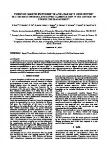
(a) Height (H)
(b) Height Variation (HV)
(c) Normal Variation (NV)
(d) LiDAR Return Intensity (LRI)
(e) Image Intensity (I)
Figure 1. The five features used in data classification for one of the training regions.
comparison of these algorithms. We have used a variation of these standard algorithms to create a terrain model from aerial LiDAR data in order to compute normalized height.
The objective of this work is to perform classification of aerial LiDAR data into 4 classes using all the 5 features or 3 classes using only 3 height-derived features. Previous classification efforts include research by Axelsson [2], Maas [13], Filin [9], Haala and Brenner [11], and Song et. al. [20]. Most of these approaches are ad-hoc heuristics. Also, in most cases results are presented for small regions without much discussion on the quality of results obtained. Finally, these approaches often require substantial manual input and sometimes tweaking of weight parameters.
Anguelov et al. [1] classify ground-based LiDAR scan points as building, tree, or shrub using a Markov Random Field model that jointly classifies data points while encouraging spatial contiguity. They report an accuracy rate of 93% for their associative Markov networks algorithm, and 68% to 73% accuracy for SVM methods on their data.
Previous work on the same aerial LiDAR data used the EM (Expectation-Maximization) algorithm with a mixture of Gaussian models [7] to classify LiDAR data into four categories. There are several differences between this previous work and our current work. The previous work required additional information – DEM data, co-registered with the LiDAR data. Also, here we use a different feature set: we introduce normal variation, which we find very useful in our classification. Finally, as reported in Section 5, we obtain higher accuracy (better than 93%) in comparison to the 66-84% accuracy reported in the previous work.
3. Data Processing
����
��� � � �� ������������� ���������� ���"!#�$���$���� ��
Our LiDAR dataset covers 8 square miles of the campus at the University of California at Santa Cruz and was collected using a 1064 nm laser at a pulse rate of 25 KHz. The raw data consists of about 36 million points with an average point spacing of 0.26 meters. We resampled this irregular LiDAR point cloud onto a regular grid with a cell size of 0.5m using nearest-neighbor interpolation. In addition, we used high resolution (0.5ft/pixel) ortho-rectified grayscale aerial imagery. To match the LiDAR data these images are downsampled to 0.5m/pixel, then registered using the NAD83 State Plane Coordinate System, California Zone III.
��&%'�)(����$��*+�,�"We identified five features to be used for data classification purposes: normalized height, height variation, normal variation, LiDAR return intensity, and image intensity.
.
.
Normalized Height (H): We computed the terrain elevation data automatically from the aerial LiDAR data using a variation of the standard DEM extraction algorithms [19]. The LiDAR data is normalized by subtracting terrain elevations from the LiDAR data.
.
Height Variation (HV): Height variation is measured within a /'01/ pixel 2436573 8:9= window and is calculated as the absolute difference between the min and max values of the normalized height within the window. Normal Variation (NV): We first compute the normal at each grid point using finite differences. Normal variation is the average dot product of each normal with
.
other normals within a �� 0 �� pixel 2�3 8 9 ; = window. This value gives a measure of planarity within the window.
.
LiDAR Return Intensity (LRI): Along with height values, aerial LiDAR data contains the amplitude of the response reflected back to the laser scanner. We refer to this amplitude as LRI. Image Intensity (I): Image intensity corresponds to the response of the terrain and non-terrain surfaces to visible light. This is obtained from the gray-scale aerial image.
Figure 1 shows images of these five features computed on the College 8 Region of the UCSC Campus. The feature values were compressed to byte values (0-255) to ease storage requirements.
�� '� �����$- -:��- ������� �,����������� We classified the dataset into 4 classes: roofs (or buildings), trees or high vegetation (includes coniferous and deciduous trees), grass (includes green and dry grass), and roads (asphalt roads, concrete pathways and soil). When using only three height-derived features H, HV, and NV, we classified the data into 3 classes by merging roads and grass into the same class. Datasets for ten different regions were segemented and some subregions were manually labeled for training and validation. The size of these labeled data sets vary from 100,000 points to 150,000 points. The mix of different classes – trees, grass, roads, and roofs – vary within these data sets. Roughly 25-30% of these data sets were labeled to cover these 4 classes adequately.
4. The SVM Algorithm Support vector machines (SVMs) are a powerful learning method that is widely used in a variety of domains. Originally introduced by Boser, Guyon and Vapnik [4], SVMs and related kernel-based methods are the subject of a large body of work in classification, regression, and clustering problems. We give only a cursory summary of the algorithm and refer the reader to any of the excellent introductions to the topic for more details (for example, Sch¨olkopf and Smola [18], Christianini and Shaw-Taylor [8], or Burges [5]). We first outline the SVM algorithm in the most basic binary classification setting and then discuss the necessary extensions for more complex prediction problems, including the LiDAR classification problem. �+����� �
�� +� *� �� ����� ��� �����$- - ���#��� ���� ��
The problem of binary classification is to use a set of training data to create a classifier which will correctly pre-
dict the label of future examples that are not present in the training set. Let ����� 2�������� � =!� 5>5 5"� 2��$#%�&�'# =)(+*-, 0/. be the 9 -example training set where each ��0 is an 1 dimensional feature vector and ��0 is an integer class label. We need only consider the case where , �32 4 ; for binary classification we use the convention that . �5��67 � ( . ��67 � ( . A binary classifier is a function 8�9:2 4A@ B 2���= � sgn 2�CED �GFIH = . If there exists C and H such that 8?>A@ B 2�� 0 = � � 0 for J��< �>5>5 5"� 9 then the training set is linearly separable. The geometric margin measures the distance from examples to the separating hyperplane of a hypothesis. The geometric margin of example 2��K��� = with respect to hypothesis >AO P�QRB 8L>A@ B is M >A@ B 2N�K��� = � � 2 S > S = . If � is incorrectly classified, then the margin is negative, and 6AM >A@ B 2N�K��� = is the distance to the hyperplane. The geometric margin of a sample �T� 2N�U�V���W�>=!�>5 5>5�� 2N�$#X�&�'# = with respect to some 8Y>A@ B is the minimum margin of any of the examples: MZ>A@ B 2 � = �\[^]`_ 0 M >A@ B 2N� 0 ��� 0 = 5 Any 8L>A@ B achieving the maximum geometric margin on a linearly separable training set is called a maximum margin hypothesis. Statistical learning theory provides evidence that maximum margin hypotheses are likely to generalize well to new data. The problem of finding a maximum margin hypothesis for a linearly separable data set is equivalent to the constrained minimization problem: a
minimize C >A@ B
= c subject to � 0 N2 C�D"� 0 FbH �
a
3
;
(1)
for JK�5 �>5 5 5`�
9 5
That is, we minimize the length of C (and thus maximize the margin) subject to the constraint that all points have distance at least 1 from the separating hyperplane. The dual of this optimization problem is h # dLe�f?g maximize 0ji ��k
0 6
subject to each 0 c k
3
h# 0 @ l i �?k � � and
0
l �'0�� l �$0$D"� l � k h# 0`i � k
(2)
0 � 0 ���
The dual form is a quadratic programming problem to which well known algorithms are applicable. In practice a specialized algorithm called Sequential Minimal Optimization (SMO) algorithm [15] is preferred due to its efficiency. �+�&%'�AmX '� �
���#����� �Wn+�o �� +� *� � �$�W� ���
The simple maximum margin framework as outlined above has three significant drawbacks which must be overcome before it can be applied to difficult classification prob-
lems like ours. First, the decision boundary of the resulting classifier, 8 , must be a linear combination of the features; second, the training set must be linearly separable; and third, only binary classification is possible. The SVM literature contains numerous solutions to these problems. High-dimensional embedding with kernels: Even if the data is not linearly separable with the original features, it may become linearly separable if new non-linear features are constructed. Thus instead of working directly with feature vector � as above, we can apply a non-linear transformation mapping � to 2N��= in a (usually much) higher dimensional space, and attempt to find a maximum margin separating plane in the higher dimensional space. Note that the dual form (2) depends on the feature vectors only through a dot product. Therefore a ker2��$0�= D 2�� l = nel function � such that � 2�� 0&��� l = � can be used to avoid the computational expense of working in the high dimensional space. Kernel functions operate directly on the original features and only implicitly represent the transformation to the highdimensional space. Two popular kernel functions are: degree- � polynomial � 2�� 0&��� l = � 2��Y0�D�� l F a �>=�
a 2�� 0&��� l = � �� �� 2 6 � � 6 �$0 ; = � Gaussian (RBF) ;�� Soft-margin classification: Even after transformation to a higher dimensional space, outliers may prevent the data from being linearly separable. In the soft-margin technique each example 2N� 0 �&� 0 = has a slack variable � 0 c � that measures how much the margin for that example falls below the desired unit distance. The primal minimization problem (1) is modified to minimize both the length of C and the sum of the slack variables: a
minimize C >A@ B�@ �
subject to � 0 �
2 � 2N�
3
a
;
0 ��C R = FbH � = c
�
F
9
h# 0`i �
�
0
6�� 0 � JK�5 �>5 5>5"�
9 �
where trades off the relative importance of slack variable minimization and margin maximization. Imbalanced data: Many classes of geographical data may be important but rare. A classifier which misses rare classes can have high accuracy but undesirable behavior. This effect was quite pronounced in our own data where, for some regions, rare classes represent only 2% of the labeled data for the region. We thus consider two different measures of accuracy for our classifier. The sample-weighted accuracy is simply the percentage of correctly classified points, this corresponds directly to the usual use of the term “accuracy”. We also consider what we term the class-weighted accuracy which splits the points into classes, computes the percentage of each class that is correctly classified, and averages these percentages. For example, consider a region that is 90% grass and 10% road and a classifier that correctly classifies
90% of the grass points but only 30.0% of the road points. This classifier has a sample-weighted accuracy of 84% but a class-weighted accuracy of only 60% on this region. In our early experiments, we observed that the � # #�� 0ji � � 0 term in the objective function tends to maximize the sample-weighted accuracy at the expense of classweighted accuracy. Our solution is to modify the slack variable term so that the under-represented class is taken more seriously. We use a set of class-specific parameters � ��� � �>5 5>5�� in the following oprimization problem: a
minimize C >A@ B�@ �
subject to � 0
2 � 2N�
a
3
0 ��C � = F �
; F
H � = c �
9
h#
����� �
0`i �
0
6�� 0 � JU� ���
�>5 5>5"�
9 5
� � 5>5>5 � The special case where � corresponds to the previous formulation. � � We must now choose each 0 . Choosing a single is difficult to do a priori, and Schoelkopf et al. propose a method to avoid doing so [17]. For our own problem we � found that the the overall parameter (or the sum of all � 0 ) made little difference. The relative weighting between classes, however, could make a large difference in classweighted accuracy for regions in which the proportion of classes in the training set was different from the test set. We hold out some data from the training set to estimate the proportions of the� various classes and then set the outlier penalty weights 0 for each class to be inversely proportional to the frequency of the class in the training set. This essentially weights the training set so that each class is equally well represented. Multiple Classes: The classifier described thus far distinguishes between two classes only; however, geographical regions are often most naturally described by more than two classes. Numerous methods are known for translating SVMs (or other binary classifiers) into a multiclass setting, including: (a) training a classifier to distinguish each class from all other classes, commonly called “One vs. All”, (b) training a classifier to distinguish between each pair of classes, or (c) using some extension of the concept of the margin to include more than two classes, and performing optimization directly on this quantity. We use a variation on (b) proposed by Wu et al. [24] which allows us to provide probability estimates for each class rather than a single hard classification. Our methodology is as follows: For each pair of classes we train an SVM on data from only those two classes. Each of these SVMs is modified so that it predicts a pair of probabilities for its two classes rather than just a single class label. When predicting the label of a new point, the algorithm takes the pairwise class probabilities from the trained SVMs and then merges them into a single distribution over all of the classes using the optimization procedure of Wu
et al. [24]. The class with the highest probability in this merged distribution is the final prediction. We use a modification of the technique proposed by Platt [14] to produce pairwise probability estimates for each of the trained SVMs. Given a road-tree classifier 8Y>A@ B that computes V>A@ B 2N��= and predicts road (� ) if �>A@ B 2N��=�� � and tree (� ) otherwise, Platt creates a function ���U@ � 2���= estimating 2�� � � � �K��� � � or � � � = by fitting the following logistic sigmoid to the data
� �U@ � 2N��= �
F
� ��
2��
�� = 5
>A@ B N2 ��=RF
The parameters � and � are fit by minimizing the negative log likelihood of the the road-tree training data: h# 0`i �
� 2N� 0 �= �����"2 ���U@ � 2N� 0 = =RF 2 6 � 2N� 0 = =������ 2 � 6 ���U@ � 2N� 0 = =
(3) where � 2 � = �5 and � 2 � = �o� reflect the class labels. Platt points out that this method has a bias problem as the same data is used to both train the SVM and to fit the sigmoid. We follow his suggestion to regularize, setting � � 2 � = ��� � QQ � and � 2 � = � where "#� is the numQ ; ; � is the number of tree � � � ! ber of road points in the data and "$ points. We found that a further modification was needed to protect the probabilities of rare classes. Therefore we adjust the likelihood function (3) by multiplying each term in the sum� � � � � � mation by (recall that is inversely proportional to the frequency of class � 0 in the training data). This correction essentially causes the likelihood calculation to act as if the two classes were represented equally in the training set.
5. Results and Discussion We use a modified version of the freely available LIBSVM [6] to test the performance of the SVM algorithm and its probablistic multiclass extensions on our LiDAR data. Figure 2 presents the accuracy results for the ten training regions using the leave-one-out test (train on the labeled subset of nine regions and test on the labeled subset of tenth region) using a radial basis function (RBF) kernel. Our RBF kernels typically used % ; � � 5 �L as the variance of the � Gaussian and 0 as inversely proportional to the frequency of that class in the given training data set as described before in Section 4.2. We have used both sample-weighted and class-weighted accuracy (described under “Imbalanced data” in Section 4.2) to assess the results. We obtained better than 90% sample-weighted accuracy for all regions and better than 90% class-weighted accuracy for 8 out of 10 regions for 5 feature 4-way classification. The other two regions have a severe data imbalance (very
Region Reg. 1 Reg. 2 Reg. 3 Reg. 4 Reg. 5 Reg. 6 Reg. 7 Reg. 8 Reg. 9 Reg. 10 Average
5 features, 4 classes class-wt sample-wt accuracy % accuracy % 74.26 93.13 92.32 94.82 94.90 95.50 93.90 96.21 94.38 95.27 92.20 90.53 91.68 91.19 92.07 94.94 73.95 90.90 95.10 95.31 89.48 93.78
3 feature, 3 classes class-wt sample-wt accuracy % accuracy % 86.61 95.40 98.09 97.84 97.14 96.05 96.54 97.95 96.22 96.39 96.25 98.52 95.66 96.92 97.90 96.52 86.17 94.55 98.83 98.91 94.94 96.91
Figure 2. Accuracy by region using the RBF (Gaussian) kernel. For each region, training was done on 150,000 points chosen at random without replacement from nine of the regions and testing was done on all labeled points in the remaining region.
few road points) that makes good class-weighted accuracy a challenge. The results for 3 feature 3-way classification are better than 94%. Previous work on the same LiDAR data using Gaussian mixture models achieved accuracy rates of 66–84% [7]. Anguelov et al. use SVMs as well as a graph cuts based algorithm to classify ground-based LiDAR terrain data [1]. They report 68% to 73% accuracy using SVM methods and 93% accuracy for their spatially coherent associative Markov Networks algorithm. Since their LiDAR data has very different properties from ours, we are reluctant to draw conclusions from these accuracy numbers. Figure 3 reorganizes our accuracy results to identify the two types of error – misclassified points by correct class (Error I) and misclassified points by prediction (Error II). These errors are less than approximately 10% for all classes for 3-way classification but higher than 10% for road and grass for 5-way classification. Road and Grass prove to be the most difficult classes to adequately seperate. This is understandable as their height information is relatively similar in many areas. We have performed extensive testing in order to determine how robust the algorithm is to changes in parameters. These include experiments with various kernel functions and their parameters, as well as more general parameters � such as variations in training data size and , which trades between margin maximization and slack variables. Figure 4 reports the results from experiments using various kernel functions. Although the Gaussian kernel was our choice and shows marginally superior performance, it is worth noting that the linear and sigmoid kernels also perform well. Indeed, linear kernels can produce far sparser kernels and thus train and classify much more quickly. This shows that it is primarily maximizing the margin rather than the high-dimensional embedding that gives the SVM high
Sample-Weighted Accuracy Vs. Training Set Size 100.00
Tree 97.03 2.31 0.87 4.27 7.44
Grass 0.37 78.31 8.94 2.53 11.83
Road 0.65 11.91 89.94 0.58 13.14
Bldg. 1.95 7.47 0.25 92.63 9.68
Error I 2.97 21.69 10.06 7.38
Road-Grass 0.77 92.45 0.38 1.15
Bldg. 3.05 6.37 96.21 9.42
Error I 3.83 7.56 3.79
80.00 Sample Accuracy
5/4 Tree Grass Road Building Error II
60.00
40.00
20.00
3/3 Tree Road-Grass Building Error II
Tree 96.17 1.18 3.42 4.60
5 features, 4 classes 3 features, 3 classes 0.00 10
100
1000
10000
100000
Training Set Size Sample-Weighted Accuracy Vs. Sigma 100.00
Sample Accuracy
95.00
Figure 3. Confusion matrices for 4 classes/5 features and 3 classes/3 features for the results presented in Figure 2. The vertical axis is the true class, and the horizontal axis is the predicted class. Type I errors are points of a given class misclassified as another; Type II errors are points misclassified as the given class.
90.00
85.00
80.00 5 feature, 4 class 3 feature, 3 class 75.00 0.10 0.20 0.30 0.40 0.50 0.60 0.70 0.80 0.90 1.00 Sigma
5 features, 4 classes Kernel Type RBF Linear Sigmoid Polynomial deg. 2 Polynomial deg. 3 Polynomial deg. 4 Polynomial deg. 5 Polynomial deg. 6
sample-weighted
class-weighted
accuracy (%) 93.78 90.67 90.20 89.03 75.71 49.90 37.47 46.63
accuracy (%) 89.48 91.56 91.18 90.01 80.62 63.66 32.91 28.92
Figure 4. Classification accuracy using different kernels: Training is done on a 100,000 point random sample from all geographical regions and testing is done on a similarly drawn disjoint sample of equal size.
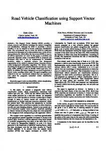
accuracy on our data. For our chosen Gaussian kernel, we also experimented with various values of % , which determines the kernel width. As shown in the lower plot of Figure 5, performance is quite stable under variations of % . The upper diagram of Figure 5 shows that acceptable accuracy is achieved even with relatively small training sets. Performance also remained quite stable under changes in � , the relative weighting between margin maximimization and the slack variables (the top plot in Figure 6) so long as it remained higher that � 5 . The stability under variations � � in the individual 0 values is slightly more complicated. In � � most published work only a single value � � 0ji � 0 is used for all classes. Both class- and sample-weighted ac-
Figure 5. (Top): Sample-weighted accuracy as a function of training set size. (Bottom): Reasonable values of (Gaussian kernel width) all give comparable results.
%
curacy � suffered when the relative proportions between the values 0 and the class proportions in the test set differed significantly (see the bottom plot in Figure 6). We show details of the visualization of classification results for one of the regions (see Figure 7). This visualization brings out the buildings (in blue), trees (in green), roads (in brown), and grass (in yellow). For the purpose of visualizing classification confidence we use the ratio of the difference between the most and next-most probable and the most probable classification to determine the saturation of each point. Thus darker points are classified with lower confidence. Areas around the edges of buildings prove to be difficult to classify. These areas have atypical coloring, and high height and normal variance, making them easily confused with trees. Cars, shrubs, and other objects for which we have no fully adequate class also frequently occur. In general we noticed that the difficulties of the classifier tend to follow the difficulties of a human classifier. Indeed many misclassifications represent truly ambiguous regions, e.g. trees which overhang buildings, or small patches of what seems to be grass or shrubs in the middle of a forested region.
Figure 7. (leftmost) Four-way classification: buildings (blue), trees (green), roads (brown), and grass (yellow); (2nd from left) Four-way confidence rated classification (darker means less confidence); (3rd from left) Threeway classification (buildings (blue), trees (green), roads and grass (yellow); (rightmost) Three-way confidence rated classification of the same region. Training for this test was done on a training set of size 150,000 points drawn randomly from the nine other regions.
6. Conclusions and Future Directions C Parameter Versus Sample-Weighted Accuracy 100.0
Sample Accuracy
90.0
80.0
70.0
60.0 5 features, 4 classes 3 features, 3 classes 50.0 0.001
0.01
0.1
1
10
100
1000
10000
C L1 Norm Versus Distance From Sample Proportions 100.0 95.0
Accuracy
90.0 85.0 80.0 75.0 70.0 65.0 0.0
Average Sample-Weighted Accuracy Average Class-Weighted Accuracy Sample-Weighted Accuracy Class-Weighted Accuracy 0.2
0.4
0.6
0.8
1.0
1.2
1.4
Distance
� Figure 6. (Top): Sample-weighted accuracy as a � � � � � � 0ji � function of overall . (Bottom): Accuracy as a function of relative entropy to the sample distribution. As proportions differ greatly from the training set accuracy declines.
We have applied the SVM algorithm to classify aerial LiDAR data and established that stable, robust, accurate classification results are achievable. Still, there are several areas of improvement worth exploring. First, spatial coherence may be used to improve the results further. One could perhaps use recently developed large-margin SVM-like algorithms which can be kernelized and work directly with a statistical model using an extended concept of the margin [21] [22]. In recent work Zabih and Kolmogorov [26] propose a segmentation algorithm that simultaneously uses both feature space and geographic space to cluster pixels and Anguelov et al. [1] learn a model that jointly classifies data points while encouraging spatial coherency. Although considering the classifications and confidences of nearby points is a powerful technique to reduce noise and outliers, this must be done very carefully in our application. Since we are interested in eventually recovering building footprints, the ”rounding” of corners could create problems. Furthermore, important details like thin road segments and small isolated buildings could be missed if one aggressively enforced spatial coherency. Second, other machine learning algorithms such as AdaBoost may also be used to obtain better or perhaps simpler and more insightful classification of aerial LiDAR data. We plan to explore these approaches in our future work.
Acknowledgements This research is partially supported by the Multidisciplinary Research Initiative (MURI) grant by U.S. Army Research Office under Agreement Number DAAD19-00-1-0352, the NSF grant ACI-0222900, and the NSF-REU grant supplement CCF-0222900.
[14]
[15]
References [1] D. Anguelov, B. Taskar, V. Chatalbashev, D. Koller, D. Gupta, G. Heitz, and A. Ng. Discriminative learning of markov random fields for segmentation of 3D range data. In IEEE International Conference on Computer Vision and Pattern Recognition (CVPR), San Diego, California, June 2005. [2] P. Axelsson. Processing of laser scanner data -algorithms and applications. ISPRS Jourmal of Photogrammetry and Remote Sensing, 54(2-3):138–147, 1999. [3] J. B. Blair, D. L. Rabine, and M. A. Hofton. The laser vegetation imaging sensor: a medium altitude, digitsation-only, airborne laser altimeter for mapping vegetaion and topography. ISPRS Journal of Photogrammetry and Remote Sensing, 54:115–122, 1999. [4] B. E. Boser, I. Guyon, and V. Vapnik. A training algorithm for optimal margin classifiers. In Computational Learing Theory, pages 144–152, 1992. [5] C. J. C. Burges. A tutorial on support vector machines for pattern recognition. Data Mining and Knowledge Discovery, 2(2):121–167, 1998. [6] C.-C. Chang and C.-J. Lin. LIBSVM: a library for support vector machines, 2001. Software available at http://www.csie.ntu.edu.tw/ cjlin/libsvm. [7] A. P. Charaniya, R. Manduchi, and S. K. Lodha. Supervised parametric classification of aerial lidar data. IEEE workshop on Real-Time 3D Sensors, pages 25–32, June 2004. [8] N. Cristianini and J. Shawe-Taylor. An Introduction to Support Vector Machines (and Other Kernel-Based Learning Methods). CUP, 2000. [9] S. Filin. Surface clustering from airborne laser scanning data sagi filin. In ISPRS Commission III, Symposium 2002 September 9 - 13, 2002, Graz, Austria, pages A–119 ff (6 pages), 2002. [10] C. Frueh and A. Zakhor. Constructing 3D city models by merging ground-based and airborne views. In IEEE Conference on Computer Vision and Pattern Recognition 2003, June 2003, 2003. [11] N. Haala and C. Brenner. Extraction of buildings and trees in urban environments. ISPRS Jourmal of Photogrammetry and Remote Sensing, 54(2-3):130–137, 1999. [12] K. Kraus and N. Pfeifer. Determination of terrain models in wooded areas with airborne laser scanner data. ISPRS Jourmal of Photogrammetry and Remote Sensing, 53:193– 203, 1998. [13] H.-G. Maas. The potential of height texture measures for the segmentation of airborne laserscanner data. 21st Canadian
[16]
[17] [18] [19]
[20]
[21]
[22]
[23]
[24]
[25]
[26]
Symposium on Remote Sensing, Ottawa, Ontario, Canada, 1999. J. Platt. Probabilistic outputs for support vector machines and comparison to regularized likelihood methods. In A. J. Smola, P. Bartlett, B. Sch¨olkopf, and D. Schuurmans, editors, Advances in Large Margin Classifiers, pages 61–74, 2000. J. C. Platt. Fast training of support vector machines using sequential minimal optimization. In Advances in kernel methods: support vector learning, pages 185–208, Cambridge, MA, USA, 1999. MIT Press. W. Ribarsky, T. Wasilewski, and N. Faust. From urban terrain models to visible citites. IEEE Computer Graphics and Applications, 22(4):10–15, July 2002. B. Sch¨olkopf, A. Smola, R. Williamson, and P. Bartlett. New support vector algorithms, 2000. B. Sch¨olkopf and A. J. Smola. Learning with Kernels. The MIT Press, Cambridge, MA, 2002. G. Sithole and G. Vosselman. Comparison of filtering algorithms. In ISPRS Commission III, Symposium 2002 September 9 - 13, 2002, Graz, Austria, 2002. J. H. Song, S. H. Han, K. Y. Yu, and Y. I. Kim. A study on using lidar intensity data for land cover classification. In ISPRS Commission III, Symposium 2002 September 9 - 13, 2002, Graz, Austria, 2002. B. Taskar, C. Guestrin, and D. Koller. Max-margin markov networks. In S. Thrun, L. Saul, and B. Sch¨olkopf, editors, Advances in Neural Information Processing Systems 16. MIT Press, Cambridge, MA, 2004. I. Tsochantaridis, T. Hofmann, T. Joachims, and Y. Altun. Support vector machine learning for interdependent and structured output spaces. In ICML ’04: Twenty-first international conference on Machine learning, New York, NY, USA, 2004. ACM Press. G. Vosselman. Slope based filtering of laser altimetry data. International Archives of Photogrammetry and Remote Sensing, 33, 2000. T.-F. Wu, C.-J. Lin, and R. C. Weng. Probability estimates for multi-class classification by pairwise coupling. In S. Thrun, L. Saul, and B. Sch¨olkopf, editors, Advances in Neural Information Processing Systems 16. MIT Press, Cambridge, MA, 2004. S. You, J. Hu, U. Neumann, and P. Fox. Urban site modeling from lidar. In Second International Workshop on Computer Graphics and Geometric Modeling, 2003. R. Zabih and V. Kolmogorov. Spatially coherent clustering using graph cuts. In CVPR, pages 437–444, 2004.