May 26, 2011 - 2Fısica Te`orica: Informació i Fen`omens Qu`antics, Edifici Cn,. Univ. Aut`onoma de .... that a privileged observer obtains the best estimate. We.
Scavenging quantum information: Multiple observations of quantum systems P. Rapˇcan1 , J. Calsamiglia2 , R. Mu˜ noz-Tapia2 , E. Bagan2,3,4 and V. Buˇzek1,5
arXiv:1105.5326v1 [quant-ph] 26 May 2011
1 Research Center for Quantum Information, Institute of Physics, Slovak Academy of Sciences, D´ ubravsk´ a cesta 9, 845 11 Bratislava, Slovak Republic 2 F´ısica Te` orica: Informaci´ o i Fen` omens Qu` antics, Edifici Cn, Univ. Aut` onoma de Barcelona, 08193 Bellaterra (Barcelona), Spain 3 Department of Physics, Hunter College of the City University of New York, 695 Park Avenue, New York, NY 10021, USA 4 Physics Department, Brookhaven National Laboratory, Upton, NY 11973, USA 5 Faculty of Informatics, Masaryk University, Botanick´ a 68a, 602 00 Brno, Czech Republic
Given an unknown state of a qudit that has already been measured optimally, can one still extract any information about the original unknown state? Clearly, after a maximally informative measurement, the state of the system ‘collapses’ into a post-measurement state from which the same observer cannot obtain further information about the original state of the system. However, the system still encodes a significant amount of information about the original preparation for a second observer who is unaware of the actions of the first one. We study how a series of independent observers can obtain, or scavenge, information about the unknown state of a system (quantified by the fidelity) when they sequentially measure it. We give closed-form expressions for the estimation fidelity, when one or several qudits are available to carry information about the single-qudit state, and study the ‘classical’ limit when an arbitrarily large number of observers can obtain (nearly) complete information on the system. In addition to the case where all observers perform most informative measurements we study the scenario where a finite number of observers estimate the state with equal fidelity,regardless of their position in the measurement sequence; and the scenario where all observers use identical measurement apparata (up to a mutually unknown orientation) chosen so that a particular observer’s estimation fidelity is maximized. PACS numbers: 03.67.-a, 03.65.Ta
I.
INTRODUCTION
One of the major questions in the interpretation of quantum mechanics is to assert the reality of the wave function. Despite the opinion galore, which also includes rejecting the necessity of attributing reality to a quantum state [1], there is a consensus in that all information on the state of a system is contained in the wave function (in the sense that it provides the right outcome probabilities for each conceivable measurement on the system). Since all this information is not accessible by a single measurement and, on top of that, quantum formalism only gives outcome probabilities, the meaning of the wave function has been traditionally associated to an infinite ensemble of identically prepared quantum systems (something which cannot be taken literally, but only as a conceptual notion). Ground-breaking experiments with individual quantum systems (see e.g. [2–5]) and the advent of quantum information technology have brought the focus to individual systems, away from the infinite ensemble picture. The inherent limitation of quantum measurements to obtain complete information about a system is intimately linked to the disturbance they cause on the state. Clearly, if a given measurement extracts the maximum information on the state of a system, then the same observer cannot obtain additional information by performing further measurements on the system. This almost tautological statement has the staring consequence that quantum measurements, no matter how cautelous they are,
inevitably disturb the state of the system (and thereby erase any information on the original state of the system as far as the same observer is concerned). The question remains: What happens if the second measurement is performed by a second observer who independently aims at gaining information about the original state of the system? Indeed, we will see that a second independent observer, who does not know the precise actions nor measurement results of the previous observers, can still obtain some information on the original state of the system. In this article will study how does this information degrade through a sequence of independent measurements performed by independent observers. We extend the study to the case where several copies of the unknown state are provided to the observers and, more generally, when several copies of the system are used to collectively encode the unknown single-copy state in more efficient ways [32]. This will allow us to give a new insight on a thorny problem in quantum mechanics, namely the so called quantum to classical transition [6]. The microscopic world is governed by the rules of quantum mechanics, which often seem to be in sharp contrast with the rules of classical physics that govern the macroscopic world. Since we both observe the classical macroscopic world and believe the quantum description is the correct one, the classical properties of systems have to appear within the quantum description in a consistent fashion. How exactly, quantitatively, do these classical properties emerge? Before attempting to answer this question it is important to recognize what are the essential features that seem to be so different in the classical and quantum
2 worlds. The problem at hand sheds some light on one of these differential aspects, which is the fragility of the information encoded in quantum states versus the enduring nature of classical information. Indeed the information encoded in a classical system can be accessed by an unlimited number of (careful) observers without degrading while quantum mechanics allows to retrieve some amount of information but this degrades as the number of observers increases. We show that the larger the number of copies of a system the more observers can gain a sizeable amount of information encoded in the original state. In other words, the information encoded in large collections of quantum systems of the same type behaves “classically”, in the sense that it is robust with respect to observations. In order to make quantitative statements we need to, first, quantify the observers’ ability to gain information about the unknown state and, second, make a judicious, precise definition of what we mean by “independent” observers. Following Refs. [7–10], we will here use as a figure of merit the quantum fidelity between unknown input (pure) quantum state ψ = |ψihψ| and the estimate, or guess, ψ ′ = |ψ ′ ihψ ′ |, that each observer arrives at, based on his measurement outcome: f (ψ, ψ ′ ) = | hψ ′ |ψi |2 . The k’th observer’s success in gaining knowledge about original system is given by the mean of the fidelity, Fk , over all possible input states and guesses: Z Fk = f (ψk , ψ0 )dp(ψk , ψ0 ), (1) where dp(ψk , ψ0 ) = dψ0 dψk p˜(ψk |ψ0 ) is the joint probability of observer k obtaining the guess ψk and the original unknown state being ψ0 , with p˜(ψk |ψ0 ) being the corresponding conditional probability density, where a uniform prior distribution for ψ0 is assumed. The integrals run over all joint events, i.e. over the set of all possible pure states ψ0 , ψk ∈ S(H). We want to define a scenario in which, one after the other, each observer gains access to the quantum system, but lacks “any” information regarding the actions of the previous observers. In principle, if no further directives are given, each observer will choose his measurement based on his own prior knowledge about it, i.e., he may describe the system as the mixed state that results from taking the original input state and performing an average over all the actions that the previous observers might have conceivably done, which includes, e.g., the obstructive action of resetting the state of the system to a fixed state. We want to find the limits on how well can independent observers recover, or scavenge, information from the very same system after successive measurements. We therefore assume that each observer will be careful, i.e. willing to facilitate the task to following observers insofar as this does not conflict with his own priorities. Accordingly, we assume that the observers are free to agree, in advance, on a protocol as long as it does not involve exchanging any information that would allow them to establish a common canonical basis, or reference
frame, in which to represent their states and actions – sharing such information would allow all the observers to perform the very same projective measurement and hence all of them would obtain the same measurement outcomes and estimate the original state with equal precision [33]. Mathematically, imposing this condition is equivalent to describing the actions of the observers in a fixed basis and then averaging the result over all possible choices of basis. More succinctly, if a given observer performs a quantum operation $ [ˆ ρ] over the system in a state ρˆ, to the other Robservers the state will effectively transform as $s [ˆ ρ] = dU U $[U † ρˆU ]U † , where dU is the Haar measure of the unitary group acting on the system’s Hilbert space. In order to complete the framework required to present all the results in this article, we still need to specify what is the figure of merit and what type of information can the observers share when several (N > 1) copies of the d-dimensional system are available. One option is to consider this multi-partite system as a single system and accordingly use the fidelity between the collective input and guess states as a figure of merit, and use the unitaries over the dN -dimensional Hilbert space in order to compute the effective transformation $s [ˆ ρ(N ) ]. However, here we will follow a different, more physically motivated, approach: Since the observers are asked to retrieve information on the encoded single-copy state, we use the fidelity between d-dimensional states, and we consider that the observers agree on using the same (mutually unknown) local basis for each of the copies, i.e. the actions of the other observers are known up to a rigid unitary operation U (g) = g ⊗N , g ∈ SU (d), i.e. the effective transformation R † † now reads $s [ˆ ρ(N ) ] = dgU (g)$[U (g) ρˆ(N ) U (g)]U (g) . This characterization of independent observers is equivalent to that encountered in protocols like aligning reference frames [11, 12] where the different parties that do not share a reference frame try to exchange some information [13]. To allow for a further generalization of this scenario we will introduce the concept of a preparer. The role of the preparer is to encode the state of a single system ψ0 = g |ψref ihψref | g † , |ψref i ∈ Hd , g ∈ SU(d) into a collective state of the Hilbert space of N by a rigid rotation Ψ = g ⊗N |Ψref ihΨref | g †⊗N , |Ψref i ∈ HD , D = dN , i.e. the signal state Ψ need not be one consisting of N copies of the initial state ψ0 , but the encoding ̺ is still covariant with respect to SU (d) and its tensor-product representation — covariant, for short. Considering covariant encodings only is actually not a restriction – as we will argue in Section III this follows from the quantum-operations averaging discussed above. The paper is structured as follows: In Section II we discuss general considerations relevant for the rest of the paper. In Section III we analyze the essential scavenging setting in which each observer maximizes the quality of its own estimate. We call this scenario the “greedy” strategy. We study the cases of: i) the optimal general encoding and ii) a symmetric encoding of the qudit state
3 into a signal state consisting of N copies of the encoded state. In Section IV we study the action of repeated weak measurements on a state. Sections V and VI are devoted to generalizations of the basic setting in which the information about the encoded state is redistributed among the observers by making use of weak measurements. We first consider what we call the egalitarian strategy, where the measurement apparata are chosen so as to provide the same quality of the estimation for all observers. We then study a complementary scenario, where all observers use the very same apparatus, but tailored in such a way that a privileged observer obtains the best estimate. We present our conclusions in Section VII. Three appendices follow with some technical details used in the main text. II.
SCAVENGING QUDIT INFORMATION: GENERAL CONSIDERATIONS
The computation of the fidelity, Eq. (1), requires the evaluation of the kth observer’s conditional probability density p˜(ψk |ψ0 ) of obtaining a guess ψk given the state to estimate ψ0 . Naturally, this quantity depends on the preparation (the way ψ0 is encoded into a signal state), on the kth observer’s measurement and the guessing strategies, and on whatever happened in-between. We may decompose each particular conditional joint event into a sum over histories — intermediate events such as measurements apparata choices, obtained measurement outcomes, or guesses made based on the outcomes — which may have led to the event (ψk |ψ0 ). It is clear that even though probabilistic strategies in the encodings and measurements choices are possible, these perform equally well as deterministic strategies which are given by averaging, with their respective probabilities, over those strategies. Without loss of generality, we may write h i ˜ (k) χk−1 ◦ . . . ◦ χ1 (̺0 (ψ0 )) , (2) p˜(ψk |ψ0 ) = Tr M ψk
where ̺0 (ψ0 ) is the state provided by the preparer, χi is a channel induced by an averaged (over all unknowns) ˜ (k) is the operator measurement of the ith observer and M density, with respect to the measure dψk , of the POVM M(k) performed by the kth observer, with measurement outcomes labeled by the guesses ψk the observer makes. Note that should several outcomes lead to the same guess, ψk , the POVM element corresponding to ψk is given by sum of all effects (i.e. POVM elements) of such outcomes. Eq. (2) can also be written as a decomposition over all intermediate observers’ guesses, ψi , Z Z h ˜ (k) p˜(ψk |ψ0 ) = dψk−1 . . . dψ1 Tr M ψk � i � (k−1) (1) × I˜ψk−1 ◦ . . . ◦I˜ψ1 (̺0 (ψ0 )) , (3)
where I˜(i) is the density of the ith observer’s average (over all unknowns) quantum instrument I (i) with mea-
surement outcomes labeled by the guesses ψi . Quantum instruments, or instruments for short, introduced by Davies and Lewis [14], are the standard mathematical tool used to describe the measurement process when one is interested not only in probabilities of measurement outcomes, but also in the post measurement state. An instrument – or an operation-valued measure – assigns to a set B of measurement outcomes an operation IB that provides a transformation rule of the state due to the measurement as well as the probability of the outcome, which is given by the trace of the transformed (postmeasurement) state. In our case, due to the limited mutual knowledge of the observer’s (and preparer’s) actions, the average instruments I (i) are covariant with respect to SU (d) and its symmetric representation U , i.e. ∀ˆ ρ ∈ S (HD ) , ∀g ∈ SU (d), (i) (i) † † I˜gψg† (ˆ ρ) = U (g) I˜ψ (U (g) ρˆU (g))U (g) .
(4)
For the same reason the (averaged) encoding ̺0 , is covariant with respect to SU (d) and its symmetric representation U , i.e. ∀ψ ∈ S (Hd ) , ∀g ∈ SU (d), †
̺0 (gψg † ) = U (g) ̺0 (ψ)U (g) .
(5)
Obviously, the channels in Eq. (2), which are induced by the instruments in Eq. (3), are also covariant with respect to U , i.e. ∀ˆ ρ ∈ S (HD ) , ∀g ∈ SU (d), †
†
χi (U (g) ρˆU (g) ) = U (g) χi (ˆ ρ)U (g) .
(6)
Subsequently, the average “encoding” χk−1 ◦ . . . ◦ χ1 (̺0 (·)) is also is covariant with respect to SU (d) and its symmetric representation U . The estimation of ψ0 can be viewed as the estimation of χk−1 ◦. . .◦χ1 (̺0 (ψ0 )) with ̺0 (ψ0 ) known to be restricted to the invariant family †
{̺0 (ψ0 ) = U (g) ̺0 (ψref )U (g) , g ∈ SU (d), U (g) = g ⊗N } (7) distributed according to the Haar measure dµ(g) = dψ0 . In other words, we have a covariant optimal estimation problem, which, with the fidelity as the cost function, can always be solved by a covariant POVM [15]. Hence, without loss of generality, we may assume the POVM M(k) to be covariant with respect to SU (d) and its symmetric representation U , i.e. ∀ψ ∈ S (Hd ) , ∀g ∈ SU (d), ˜ (k) (gψg † ) = U (g) M ˜ (k) (ψ)U (g)† . M
(8)
Eqs. (2) and (3) tell us how to proceed further. We search for pairs of covariant encodings ̺0 and POVM(s) M(1) fulfilling a desired property of the average fidelity F1 (e.g. maximizing F1 , possibly given additional constraints) for the invariant family of states Eq. (7). Having at least one such pair {̺0 , M(1) }, one can evaluate F1 . Next, for each possible POVM M(1) , obtained in the previous step, consider all covariant quantum instruments I (1) compatible with the POVM, and calculate
4 the set of covariant channels χ1 which are induced by any of those instruments. Next, search for covariant POVM(s) M(2) fulfilling a desired property of the average fidelity F2 for the average states from the covari† ant families {χ1 (̺0 (ψ0 )) = U (g) χ1 (̺0 (ψref ))U (g) , g ∈ ⊗N SU (d), U (g) = g }, distributed as governed by the Haar measure dµ(g), given by the actions of all channel(s) χ1 from the previous step, and so on. The task is greatly simplified by the possibility to restrict oneself to covariant apparata and channels. If the optimal covariant apparata turn out to be unique at each step, the task becomes even simpler. But, even in this case, one has still to calculate the induced channel at each step to obtain the set of average states for the next optimization. In the following sections we will study various scenarios which we separate in two groups: those which require maximally informative measurements, where the action for each observer can be interpreted as a measure and prepare channel; and those where the conditions of the problem require that the observers perform weak measurements extracting less information from the system.
III.
GREEDY STRATEGY
Let us now specialize to the case of ’greedy’ observers who primarily want to maximize the fidelity of their own guesses. This is precisely the main scenario that motivates this work [34]. Here the task at hand can be reduced to the problem of a preparer and single-observer encoding/estimation of quantum states embedded in larger systems. Solutions to the latter problem are often known ([7, 8, 15–18]). In this scenario, each observer performs the best estimation he can —in other words, there exists no additional measurement he could perform that would increase the fidelity of his guess, which was obtained based on his original measurement. It follows that the postmeasurement state after the ith measurement can depend on the original state ψ0 only indirectly, through the obtained guess ψi , hence the corresponding instrument can be viewed as a measure-and-prepare channel. Thus, we can rewrite the Eq. (3) in a factorized form p˜(ψk |ψ0 ) =
Z
dψk−1 p˜(ψk |ψk−1 ) . . . Z . . . dψ0 p˜(ψ1 |ψ0 ),
F (k) =
1 [ 1 + (d − 1) dZ
×
dψ0 dψk n(ψk ) · n(ψ0 )˜ p(ψk |ψ0 ) ] (11)
where n(ψ) stands for the generalized Bloch vector of a pure state ψ ∈ S(Hd ) (see Appendix A for details). As we argued in Section II, the average instrument I (i) and thus the induced POVM M(i) and the encoding ̺i , i < k, are covariant, while the POVM M(k) can be chosen to be covariant. Hence, without loss of generality, we may restrict our attention the optimal covariant POVMs for the set of equiprobable states of the invari† ant family {̺i−1 (ψi−1 ) = U (g) ̺i−1 (ψref )U (g) , ψi−1 = † ⊗N gψref g , U (g) = g , g ∈ SU (d)}. For such a situation, we show in Appendix A that Z dψi−1 n(ψi−1 )˜ p(ψi |ψi−1 ) = ∆i n(ψi ), (12) where ∆i is a number. In other words, after the measurement of the ith observer, the output state will be characterized by a “shrinked” version of the input Bloch-vector. Plugging Eqs. (9) and (12) into Eq. (11) we have ! Z k Y 1 (k) ∆i dψk n(ψk ) · n(ψk ) 1 + (d − 1) F = d S i=1 ! k Y 1 (13) ∆i . 1 + (d − 1) = d i=1 Thus, successive maximizations of F1 , F2 , . . . , Fk are achieved via successive maximizations of ∆1 , . . . , ∆k . The maximization of ∆i is over the pair – covariant encoding ̺i−1 , covariant POVM Mi for the set of states {̺i−1 (ψi−1 )} with unknown, hence equiprobable, previous observer’s guess ψi−1 = |ψi−1 ihψi−1 | ∈ S(Hd ). If the initial encoding ̺0 has been optimal, then one cannot achieve a better performance than if we take ∀i, ̺i ≡ ̺0 , i.e. ∆i = max ∆1 =: ∆. Hence, the maximum Fk of the average fidelity Fk if all Fi , i < k are, one-after-another, maximal, reads Fk =
(9)
with ˜ (i) (ψi )̺i−1 (ψi−1 )], p˜(ψi |ψi−1 ) = Tr[M
Using the Bloch-vector formalism we may rewrite the average fidelity Eq. (1) as
(10)
where ̺i−1 (ψi−1 ) is the post-measurement state after the (i − 1)th measurement given the obtained guess has been ψi−1 .
� 1� 1 + (d − 1)∆k . d
(14)
The situation is different if the initial encoding has been restricted by some additional requirements, e.g. encoding into copies of the state ψ0 , which turns out to be a suboptimal encoding with ∆sym . Then, for i ≥ 1, the best strategy is, naturally, to take ̺i equal to the unrestricted optimal ̺0 . That is, for the problem of k greedy observers independently estimating N copies of an unknown state the fidelity will read Fk =
� 1� 1 + (d − 1)∆sym ∆k−1 . d
(15)
5 In the following subsections we give the explicit expressions for the fidelity Fk for some relevant cases, which amounts to solving the relatively straightforward the single-observer problem (i.e. computing ∆). A.
The Fidelity for the optimal N -qubit encoding
Here, we treat the optimization of the qubit state encoding with full generality. The optimal encoding of a single qubit state (or, equivalently, of a spatial direction corresponding to a spin-1/2 particle) into U -invariant family of N -qubit states is given by Bagan et al. in Ref. [16]. The optimal signal state (k = 0) as well as the state prepared after the kth measurement, k > 1, reads †
̺k (mk ) = U (mk ) |AihA| U (mk );
k ≥ 0,
where xN/2+1 is the largest zero of the Legendre polynomial PN/2+1 (x). Thus Fkop =
xn = 1 −
X j=0
Aj |j, 0i,
(for simplicity we assume that N is even) with the coefficients Aj such that |Ai is the eigenvector corresponding to the maximal eigenvalue of the matrix 0 cl−1 0 . . . 0 . cl−1 . . . . . . . . . .. .. .. , (17) 0 . . c2 0 . .. .. . c2 0 c1 0 · · · 0 c1 0
where
l=
N +1 2
(18)
ξ02 + ··· , 2n2
(24)
where ξ0 = 2.4 is the first zero of the Bessel function J0 (x). Hence, asymptotically (for N → ∞), ∆∼ =1−
2ξ02 , N2
(25)
and
(16)
N/2
(23)
Asymptotically, it is known that
Fkop
where |Ai =
i 1h 1 + xkN/2+1 . 2
" � � # 2 k 2ξ 1 ∼ 1 + 1 − 02 . = 2 N
(26)
In the case where the signal state is given as N copies of the unknown state, i.e. ψ0⊗N , the first (k = 1) shrinking factor needs to be replaced by that of the well known N -qubit pure state estimation ∆sym = NN+2 (see next subsection for general qudit derivation). So that, � � N 1 N copy k−1 1+ (27) x Fk = 2 N + 2 N/2+1 " # � �� �k−1 1 2 2ξ02 ∼ 1 + 1 − 1 − . (28) = 2 N N2 We note that by allowing operations to act on the whole Hilbert space of N qubits provides a significant advantage with respect to strategies relying on the encoding into N copies, ψ0⊗N , (which lies the in completely symmetric subspace): in the latter case the maximum fidelity is approached as 1/N , in contrast to the 1/N 2 behaviour found in the optimal case — see end of this Section for a more detailed discussion.
and i ci = p . (2i + 1)(2i − 1)
(19)
The operator density of the corresponding optimal measurement can also be found in [16]: M (k) (mk ) = U (mk ) |BihB| U † (mk );
k > 1,
(20)
where N/2
|Bi =
Xp 2j + 1|j, 0i.
(21)
j=0
In this case ∆ = xN/2+1 ,
(22)
B.
The Fidelity for N parallel qudits
For general d-dimensional states the general optimization is a hard problem to solve. In this section we will limit ourselves to the situation where the measurement apparata of the different observers are restricted to operate in the Hilbert space of the initial state, which we also take to be N copies of an arbitrary pure qudit state. That is, during the whole measurement sequence the system will be constrained in the totally symmetric subspace of the state space S(HD ). A natural way to impose this limitation could be to require that if in the fortunate, but ‘extremely rare’, event that an observer guesses the input state correctly, then the output state should be left in exactly the same collective state as the input.
6 The POVM M = Msym optimal for the encoding into copies is known to be the extremal covariant POVM [15] with the operator density on the relevant, symmetric, subspace given by
For smaller sizes N ∼ k α with α < 1 the fidelity inevitably drops to that of the random-guessing strategy,
˜ sym (ψ) = dsym |ψihψ|⊗N M N
For the optimal recycling of information, we see that, for qubits,
(29)
Fk →
where ⊗N
|ψi
⊗N
= (g |ψref i)
, g ∈ SU (d), |ψref i ∈ Hd . (30)
The maximal single-observation fidelity is Z ˆ N |2 p(ψ|ψ) ˆ dψdψˆ |hψ|ψi F1sym = Z sym = dN dψ |hψ|ψref i|2(N +1) �Z sym = dsym hΨ | dµ(g) U(g) N ref � sym
sym † ×|Ψsym ref i Ψref |U(g) |Ψref i =
dsym N , dsym N +1
(31)
⊗(N +1) where |Ψsym , and the dimension of the ref i = |ψref i completely symmetric representation is given by � � N +d−1 dsym = . (32) N N
Substituting Eq. (32) into Eq. (31) we get F1sym =
N +1 . N +d
Using Eq. (14) we have " � �k # N 1 sym 1 + (d − 1) Fk = d N +d " � �k # 1 d ∼ 1 + (d − 1) 1 − , = d N
(33)
(34) (35)
where the approximation holds in the asymptotic limit of large number of copies. From the above results we can readily obtain some conclusions on how large a system needs to be in order to be considered “classical” as far as the readout of the information is concerned. The minimum size N is related to the number of independent observations we may perform on it and still get good estimates. For parallel spins, we see that we need a minimum size of the order N ∼ kα ;
α>1
(36)
if we wish to obtain the classical behavior Fk → 1.
(37)
Fk → 1
1 . 2
if N ∼ k α , α > 1/2,
(38)
(39)
hence, in this case we just need a size square root of the number of observations for a system of spins to be considered classical. Note that the above is not in contradiction with the result [19] where the authors obtain k = O(N 2 ) for what we call symmetric encoding into parallel spins. The quantity considered in [19], related to longevity, k, of a directional reference carried by a quantum system, is the first moment of the spin-projection operator for the state after � k uses, Jn(ψ) ρ (ψ) = (2Fk − 1)(N + 2)/2, which they k require to stay above arbitrary but fixed threshold c. We require that the threshold approaches (N + 2)/2 for all N and we take the limit N → ∞. IV.
WEAK MEASUREMENTS
We aim now to generalize the problem to situations where the observers do not pursue the mere maximization of their estimation fidelity, but adopt strategies where the information on the unknown state is redistributed in different ways among the various independent observers. In the following sections we will study the case where K observers estimate the original state with equal, but maximal, fidelity (egalitarian strategy) and the case where all observers use the same measurement apparatus and the goal is to optimize the estimation fidelity of the kth observer. In both instances the measurements performed need to be weak, i.e. in general not extracting all of the extractable information and hence inflicting less disturbance to the state. As in the greedy-observers scenario, it suffices to consider covariant measurements. All U covariant POVMs (with outcomes labeled by the guesses) have operator density of the form † ˜ M(ψ) ∼ U (g) Sref U (g) ,
(40)
ψ = gψref g † , U (g) = g ⊗N , g ∈ SU (d),
(41)
with
where Sref can be a positive operator commuting with {U (g) ; g ∈ Gref }, where Gref ⊂ SU (d) is the set of unitaries which leave the reference state ψref invariant [15] — the completeness POVM relation can be easily imposed in this covariant construction. It is clear that, for optimal weak measurements, the post-measurement states will not in general be pure anymore. They will depend not only on the measurement
7 outcome (guess) of the current observer but on particular guesses of all predecessing observers and the preparation parameter ψ0 . The probability density of obtaining measurement outcome leading to a guess ψk , given the previous observer has obtained the guess ψk−1 , is not independent of previous observers’ guesses, i.e. p˜k (ψk |ψk−1 , . . . , ψ0 ) = p˜(ψk |ψk−1 ) does not hold in general. Thus, we have to start with the histories decomposition Eq. (2) since Eq. (3) does not simplify to Eq. (9) anymore. To proceed further, we will hence follow the approach outlined in Eq. (2), where to the kth observer, the action of all previous observers is described as covariant channels. We hence need to calculate actions of the channels χk , k = 1, . . . , K − 1. We will do that in what follows for the single qudit case and for the qubit case restricted to encoding into copies.
A.
Single copy: arbitrary dimension
We start with the case of a (single copy) of an unknown pure state ψ0 = |ψ0 ihψ0 | of arbitrary finite dimension d. A qudit being measured using a SU (d)-covariant instrument undergoes, if the measurement outcome is unknown, the dynamics given by the channel χk which is SU (d)-covariant, i.e. a convex combination of the identity channel and the contraction to the total mixture, acting as χk (ˆ ρ) = rk ρˆ + (1 − rk )1/d.
(42)
On the other hand, the kth observer’s fidelity of the guess of an original reference state ψref , for an effectively en(k−1) coded state ρˆref = χk−1 ◦ . . . ◦ χ1 (|ψref ihψref |) – the result of sending |ψref ihψref | through the SU (d)-covariant channels χ1 , . . . , χk−1 – is given by Fk =
XZ o
� � dµ (g) Tr g |ψref i hψref |g † go |ψref i hψref | go†
i h (k−1) × Tr g ρˆref g † Mo(k) ,
(43)
where the state we wish to estimate is g |ψref ihψref | g † . For convenience, we assume the (currently) last observer’s POVM to be one with finitely many outcomes denoted by o. The guess associated with an outcome is denoted by ψo = go |ψref ihψref | go† . Using Eq. (C1) of Appendix C we obtain (k−1)
Fk =
(k−1)
where OS
(k)
(k−1)
− 1)OM (dOS d − OS + , d(d + 1)(d − 1) (d + 1)(d − 1)
(44)
is the overlap of the states (k−1)
OS
h i (k−1) = Tr ψref ρˆref ,
(45)
(k)
and OM is the overlap between guesses and corresponding POVM elements i X h (k) (46) OM = Tr ψo Mo(k) . o
For a general SU (d)-covariant qudit channel, Eq. (42), induced by the kth measurement and the averaging due to lack of knowledge about it, one trivially has XZ Fk+1 = rk dg Tr [g |ψ0 i hψ0 | q
†
×g gq |ψref i hψref | gq† ] i 1−r h k (k−1) × Tr g ρˆref g † Mq(k+1) + d � � 1 1 = rk F − + , d d
(47)
where F is the average fidelity of the (k + 1)th observer’s guess if the measurement would have been performed on the state ρˆ(k−1) – i.e. as if the kth observer would have not measured at all. The fidelity has the property 1/d ≤ F ≤ 1, where F = 1/d corresponds to pure guessing without actually measuring anything. It follows that in order to maximize the possible Fk+1 for any fixed measurement M (k+1) one has to have rk as large as possible. Naturally, rk will be ultimately limited by the achieved Fk but also by particular choice of the kth observer’s measurements (instrument) attaining that value of the fidelity. At this stage we have to be more explicit in describing the observers’ measurement apparata. In particular we have to specify the instrument realizing the POVM M (k) that appears in Eqs. (43) and (46). Here, we have two options: The first option is that the quantum operation performed, upon obtaining any outcome o, is given by a single-term Kraus decomposition. That is the unnormalized post-measurement state for an outcome o is given by ρˆpost = A†o ρˆin Ao (we omit the index indicating the outcome in the post-measurement states). The second option is that there exist some outcomes for which the operation has multiple Kraus operators in its decomposiP † ρˆin Bα,i ; n > 1; ∀i, Bα,i 6= ˆ0,). tion (∃α : ρˆpost = ni=1 Bα,i In the latter case we formally redefine the POVMs used in Eqs. (43) and (46) – we simply use the language of the ′ := fine-grained measurement with POVM elements Mα,i † † Bα,i Bα,i and operations defined by ρˆpost = Bα,i ρˆin Bα,i for all αs where a multi-term Kraus decomposition would otherwise take place. Since the additional labels i are not used for anything (they are not accessible to the observer and thus can’t influence his guess), these new formal apparata provide an equivalent description. Thus, we can always assume a description of the measurement process in terms of an apparatus with single-term Kraus decomposition for each outcome. For such apparatus, the averaged effective channel is of the form Eq. (42), with the parameter rk acquiring a particularly simple form (see
8 Appendix C) rk =
2 X c−1 , where c = Tr A(k) o . (d + 1)(d − 1) o
(48)
Recall that we wish to have rk as large as possible given the kth observer’s achieved fidelity Fk , i.e., in the language of the single-Kraus-term apparata, the value of c as large as possible. For a given value of Fk , a measurement both reaching (k) Fk , i.e. the required OM in Eq. (44), and maximizing c in Eq. (48), is known to be given by [20] s s (k) (k) OM d − OM A(k) = |aiha| + (1 − |ai ha|) , (49) a d d(d − 1) where {|ai}da=1 is an arbitrary orthonormal basis. Thus (k) the largest c, given Fk (i.e. given OM ), is �2 �q q (k) (k) OM + (d − 1)(d − OM ) . c=
(50)
The corresponding POVM reads
=
(k−1)
Fk =
− 1)εk 1 (d OS + d d(d + 1)
(55)
and from Eq. (42) with a pure initial state, Eq. (45) reads (k)
k 1 d−1 Y + rβ . d d
(56)
β=1
(k) OM
d− −1 |aiha| + 1, d−1 d(d − 1)
(51)
i.e. for this particular POVM the optimal instrument in terms of Kraus operators is given by the Hermitian q (k)
(k)
(A˜ is the operator density of the Kraus operator [35] √ � √ A, i.e. A dψ = dψ A˜ψ ), we may verify that for a given value of Fk it induces the same channel as the minimal optimal measurement, Eq. (49). Thus, the Hermitian-square-root realization of the general weak covariant POVM, Eq. (52), gives the optimal covariant instrument. Using Eqs. (53) and (44) we have
OS =
Ma(k) = Aa(k)† A(k) a (k) OM
of the kth observer’s measurement. Constructing the corresponding Hermitian-square-root Kraus operators A(εk ) defined by q (k) OM(εk ) |ψihψ| A˜(εk ) (ψ) = s (k) d − OM(εk ) + (1 − |ψi hψ|) , (54) (d − 1)
Ma . One could continue the square-root Aa = analysis using the (unaveraged) d-outcome measurement, Eq. (49), optimal for any achievable value of Fk . However, we will proceed in terms of the effective, averaged, covariant apparata with measurement “outcomes” given by the possible guesses. Covariant apparata may be easily constructed — this is a much harder task in the case of discrete apparata for encodings into higher-dimensional Hilbert spaces (c.f. [17] for N copies of a qubit). It follows from Eq. (40) that any SU (d)-covariant POVM on a qudit (with outcomes corresponding to guesses) has the operator density of the form ˜ (εk ) (ψk ) = (1 − εk )1 + εk M(ψ ˜ k ), M
(52)
˜ is the operator density of the optimal covariant where M POVM of the greedy-observers scenario, Eq. (29), and εk parametrizes the strength of the measurement. Then, Eq. (52) leads to (k)
OM(εk ) = 1 + εk (d − 1),
(53) (k)
where we have used Eq. (46) in the form OM(εk ) = i h R ˜ (εk ) (ψk ) . Note that 1 ≤ O(k)(ε ) ≤ d, dedψk Tr ψk M M k pending on the “greediness”, or strength, εk , 0 ≤ εk ≤ 1,
Substituting the above equation into the Eq. (55) we finally obtain k−1 1 εk (d − 1) Y Fk = + rβ . d d(d + 1)
(57)
β=1
where the rβ can be expressed as function of the parameter εβ by making use of Eqs. (48), (50) and (53), p p d − 1 + (2 − d)εβ + 2 1 + εβ (d − 1) 1 − εβ . rβ = d+1 (58) The above equation applies to general consecutive measurements on a d-dimensional system (single copy). Naturally, here we recover the results of the greedy scenario, Eq. (34) with N = 1, in the limit of most-informative measurements (εk = 1). We next discuss the weak measurement case for N copies of a qubit state. B.
N copies of a qubit
Here we consider a signal that is a state of N copies of a two-dimensional unknown pure state. Again, we will assume that the observers measurements are restricted to the completely symmetric Hilbert space. Hence, this situation can be mapped to the problem of estimating the state of a single D-dimensional system (D = dsym =N+ N 1) which is, however, known to belong to the restricted
9 set of states from the orbit of a reference pure N -copy state generated by elements of the range of the symmetric representation of SU (2). It turns out to be very useful for our purposes to recall an old result by Holevo [15]. He solved the unconstrained, or in our terminology greedy, optimization problem for generic mixed states ̺(ψ) drawn from a covariant family of states � ̺(ψ) = U (g)̺(ψref )U (g)† , U (g) = g ⊗N , g ∈ SU (2) , � � (59) where ∀g ∈ SU (2) : [g, ψref ] = 0 ⇒ g ⊗N , ̺ (ψref ) = 0. He finds that the optimal fidelity F (̺) is given by
� ! 2 Jn(ψref ) ̺(ψ ) 1 ref 1+ , (60) F= 2 N +2 where � �
� Jn(ψ) ̺(ψ) := Tr Jn(ψ) ̺(ψ) ,
(61)
and Jn(ψ) is the angular moment component in the direction fixed by the Bloch vector n(ψ). The optimal greedy covariant POVM is also proven to be given by ⊗N ˜ M(ψ) = dsym independently of a particular N |ψihψ| family Eq. (59). The most general covariant POVMs one should consider here is one which has a seed that commutes with Jn(ψref ) [15], i.e., the seed is diagonal in the {|jmi} basis (where we have chosen n(ψref ) as our quantization axis). Note that, in principle, several weakness parameters could be included in the optimization, in contrast to the single parameter required in the previous subsection. Here we will make the simplifying assumption of considering single parameter families of POVMs. That is, the measurement is given by a covariant POVM that, as before, is a convex combination of the optimal greedy POVM and the full identity, i.e. ˜ (k) (ψ), ˜ (k),εk (ψ) = (1 − εk )1 + εk M M
(63)
where √ 1 − εk , q = 1 + (dsym N − 1)εk − ak .
Fε1k =
(1 − εk ) + εk F1 2
(66)
Then by Eq. (60), for an arbitrary family of states Eq. (59),
� ! 2 Jn(ψ) ̺(ψ) 1 εk 1 + εk . (67) F1 = 2 N +2 Appendix B gives us the post-measurement states for each step in a sequence of weak measurements given by Eq. (63) and thus, for each k, we can evaluate the average fidelity of the kth observer Fkε where ε = (εk , . . . , ε1 ). Formally this is done according to Eq. (67) with ̺(ψ) 7→ ρˆεk−1 = χεk−1 ◦ . . . ◦ χε1 (̺(ψ)), i.e. ! 2 hJn iρˆε 1 k−1 εk ε ε 1 + εk , (68) Fk = F1 (ˆρk−1 ) = 2 N +2 where the following relation holds between the consecutive output states (Appendix B), � � b2k+1 j 2ak+1 bk+1 hJz ik+1 = a2k+1 + hJz ik . + 2j + 1 (j + 1) (2j + 1) (69) We are now in position to calculate two interesting scenarios where weak measurements need to be considered.
(62)
˜ (k) given above, 0 ≤ εk ≤ 1 parametrizing where M the strength of the kth observer’s measurement, and (ii) with the corresponding Hermitian-square-root Kraus operators densities: ˜ (k) (ψ) M A˜(k),εk (ψ) = bk + ak 1, dsym N
although the above two restrictions seem to be a reasonable guess for a generalization of the optimal apparatus from the single-copy case, we do not have a proof that, for N > 1, such apparata really are among the optimal ones. Therefore, it is only guaranteed that we obtain a lower bound Feq on the maximum Feq , i.e. Fk ≤ Feq . We start by rewriting the average fidelity Fε1k of single estimation using the (εk -strong) apparatus, Eq. (62), of the kth observer’s measuring on arbitrary set of states in terms of estimation fidelity, F1 , obtained using the apparatus of the greedy observers problem,
ak =
(64)
bk
(65)
It is shown in Appendix B that such evolution leads to a channel that leaves the post-measurement state, after averaging over guesses, diagonal in the {|jmi} basis, and hence it is of the form Eq. (59). We emphasize that
V.
EGALITARIAN STRATEGY
We devise a protocol such that the estimation fidelity obtained by each observer is the same and maximal, i.e. we want to find the maximum fidelity, Fk ≡ Feq , under the egalitarian constraints Fk = F1 , ∀k ∈ {2, . . . , K}. The overall number of observers, K, is fixed beforehand and each observer knows his tally number k in the sequence. One can visualize this scenario as different apparata being delivered to the observers by an external party, or as observers sharing a single apparatus which adjusts its measurement-strength automatically before each measurement. We again require that each observer orients his apparatus independently, and do not allow communication between observers. With these conditions, it is clear that the last observer will perform an optimal greedy measurement for the ensemble of states on the input of his apparatus, while going
10 backwards each of his predecessor’s measurement will be weaker and weaker, i.e. less and less demolishing. With these considerations in mind we can give the results for the two types of encodings discussed in Subsections IV A and IV B. A.
System of arbitrary dimension (single copy)
Using Eq. (57) the condition Fk = Fk−1 translates into εk−1 = εk rk−1 ,
(70)
or, more explicitly through Eq. (58), εk (d + 1) p , √ d − 1 + (2 − d)εk + 2 1 + εk (d − 1) 1 − εk (71) where the initial condition εK = 1 follows from the fact that, as mentioned above, the last, Kth, observer can measure greedily as there is no subsequent observer to care about. The recursion relations Eq. (71) are quadratic and hence can be inverted analytically, providing all the measurement strengths εk starting from εK = 1. However, a closed-form solution for ε1 seems to be hard to obtain for finite K. Nevertheless, for large K we can obtain an asymptotic analytical expression of the fidelity and the initial εk ’s. If K ≫ 1 we expect the first measurements to be very weak, i.e. with εk ≪ 1. Performing a Taylor expansion around εk = 0 in the recursion relation Eq. (71) we obtain an approximated relation for small values of k εk+1 =
εk+1
(73)
(N +
−2
+ 1) + 2α (j0 )
2 (d + 1) , jd2
(75)
(76)
where j0 is a fixed (j0 ≪ K) lower boundary of integration chosen such that the above approximations are valid. With this we finally arrive at r 1 2(d + 1) ε1 = α(K) ≃ , (K ≫ 1). (77) d K Inserting the above into F1 of Eq. (57) we have, for large K, the maximal average fidelity of each egalitarian observer s " # d−1 1 2 1+ . Feq (K, d) ≃ d d (d + 1)K
(78)
Let us note that a related problem of information/disturbance trade-off in sequential weak measurements on a qudit signal has been studied in Ref. [21]. There, users are not considered fully independent, in particular they share a reference frame, which allows them to obtain an estimation fidelity that does not decrease with the number of users.
N copies of a qubit
εk hJn iρˆε
k−1
which holds for large values of j. In this regime α(j) is vanishing small and the difference equation can be written as an ordinary differential equation
1)2
(j − j0
From Eq. (68) it follows that in order for every observer to have the same fidelity (Fkε = Flε , ∀l, k s.t. 0 < l < k ≤ K), it must hold that
d2 α(j + 1)3 , 4 (d + 1)
εk+1 =
≃
s
2 ) d2 / (d
(72)
or, by defining α(j) = εK+1−j ,
dα(x) d2 =− α (x)3 dx 4 (d + 1)
α (j) =
s
B.
d2 = εk + ε3 , 4 (d + 1) k
α(j) = α(j + 1) +
which yields,
(74)
= εl hJn iρˆε
.
(79)
To proceed further we need to evaluate how the channels χεk transform hJn i for the relevant states, which we do in Appendix B. Comparing Eq. (79), with l = k + 1, to Eq. (B11) of Appendix B we get a recursion relation for the strength parameters εk :
(N + 1)(N + 2)εk p , + (N − 1)(1 − 2εk ) + 4 (1 − εk )(1 + N εk ) − 2
where εK = 1. Again, this recursion relation gives all the strength parameters εk starting on reverse from k = K.
l−1
(80)
To obtain the fidelity one needs to solve the recurrence
11 relation Eq. (80) for k = 1, and then use Eq. (68) to get 1 2
Feq (N, K) = (1 + ∆eq ) ,
(81) ∆=
where ∆eq = ε1 (K, N )
N . N +2
(82)
The presence of the square roots in Eq. (80) prevents the existence of a closed expression for ε1 . However in the asymptotic regimes of large K or large N we can find the leading order behaviors of ε1 and Feq . Let us first consider the situation K ≫ N . As above, we expect the first measurements to be very weak, i.e with εk ≪ 1, k ≤ k0 ≪ K. Thus we can do a Taylor expansion in ε around the point ε = 0 in Eq. (80) and get the approximate relation εk+1 = εk +
which yields
N +1 3 ε , 2(N + 2) k
(83)
N . N + 2K
(88)
and, clearly, for K ≫ N ∆ → N/ (2K). Note in addition that Eq. (88) is precisely the result that one obtains with a strategy where each observer performs a ˜ = N/K of the greedy measurement on a fraction N copies. Indeed from Eq. (33) with d = 2 one has ˜ /(N ˜ + 2) = N/(N + 2K). ∆eq = N Now we proceed to study the case where the number of copies is asymptotically large, i.e. N ≫ 1. The large-N expansion in Eq. (80) yields
εk+1 = εk +
2ε2k , N
(89)
which, proceeding as in Eqs. (72)-(77), leads to ε1 ≃
s
N +2 , (N + 1)K
which, starting from εK = 1, gives at the order 1/N (K ≫ N ) .
(84) ε1 = 1 −
Inserting Eq. (84) into Eq. (82), we have N , ∆eq ≃ p (N + 1)(N + 2)K
(K ≫ N ).
The condition Eq. (79) then leads to the recurrence relation that can easily be solved and gives N/2 + 1 N +2 → ε1 = , N/2 + K − k + 1 N + 2K
(90)
(85)
Again we obtain√a behaviour for large number of observers as ∆ ∼ 1/ K. This result deserves some comments, since one would naively expect that ∆ degrades with the inverse of the number of observers, i.e. as ∆ ∼ 1/K. The realization of the POVM Eq. (62) as an instrument given by Hermitian-square-root Kraus operators, Eq. (63), is crucial to obtain this square root degradation. Had we used a more destructive realization, we would indeed have obtained ∆ ∼ 1/K. For instance, if we realize the POVM Eq. (62) as a stochastic measurement such that with probability (1 − εk ) the outcome is just guessed, i.e. nothing is done to the state, and with probability εk the optimal greedy covariant measurement is performed, the (relevant part of the) channel induced by such measurement is χ′εk = (1 − εk ) Id +εk χ, where Id is the identity channel and χ is the channel induced by the optimal greedy measurements. In this case � � εk+1 hJn ik . (86) hJn ik+1 = 1 − N/2 + 1
εk =
2 (K − 1) . N
(87)
Hence, from Eq. (82) we have for N ≫ K 2K N +2 2K ≃ 1− . N
∆eq ≃ 1 −
(91) (92)
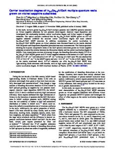
Naturally, for K = 1 in Eq. (91) we recover the well known result of the optimal measurement of N copies of a qubit [7, 22] given by Eq. (34), d = 2, k = 1. The efficiency of this egalitarian strategy in the N ≫ K regime coincides with the stochastic strategy, Eq. (88), and the a greedy one where each observer measures only ˜ = N/K of the copies. the fraction N In Fig. 1 we plot the observers’ performance ∆eq obtained by a numerical evaluation of the exact recurrence relation, Eq. (80), as well as the approximations of the limiting regimes discussed above. N = 103 has been chosen to accommodate all the regimes. The stochastic strategy performance, [Eq. (88)], which coincides with the greedy one over N/K copies, is also plotted for reference. Notice that it gives a very good approximation to the true values of the fidelity even for K & N . The deviation starts to be appreciable only beyond K ≃ 104 .
12 Deq HK,103 L
lor expanding ∆K of Eq. (93) around ε = 0 we have
1
∆K 0.1
0.01
� �K−1 d2 ε2 ε 1− = d+1 4 (d + 1) � � ε d2 K 2 ≃ e xp − ε . d+1 4 (d + 1)
(95)
The value of ε∗ that maximizes the above expression is r 2 (d + 1) ∗ , (96) ε = 2d2 K
0.001
K
which inserted in Eq. (95) yields s 2 FIG. 1: The observers’ measurement performance, ∆eq , as a ∆K,max ≃ function of the number of observers, K. Solution given by the e (d + 1) d2 K 104
100
106
exact recurrence relations [Eq. (80)], (circles). Approximate solution for K ≫ N [Eq. (85)] (dotted) and N ≫ K [Eq. (91)] (dashed). Stochastic strategy [Eq. (88)] (solid). The solid line also depicts the performance of each observer measuring only ˜ = N/K of copies. a fraction N
PRIVILEGED OBSERVER STRATEGY
Here we consider a scenario where all observers use exactly the same measurement device (up to the unknown relative orientation), but this is provided, or tailored, by a particular, say the K th, observer who wants to optimize his own estimation fidelity. That is, he has to find the right compromise, i.e. the optimal measurement strength ε, between these two extreme cases: i) choose a very weak measurement that prevents the (K − 1) previous observers to extract much information from the state and thus facilitate little disturbance, but at the same time prevents him to gain information about it when his turn comes; 2) choose the most informative measurement that will guarantee that he extracts the maximum information from the states he receives but, by then, all the previous most informative measurements will have significantly ruined the input state.
A.
For one copy, covariant POVMs with Hermitiansquare-root update rule are optimal. They are of the form of the one-parameter family given by Eq. (52). Based on Eq. (57), the fidelity FK = (1 + (d − 1)∆K )/d of the last observer is determined by ε K−1 r , d+1
(97)
N copies of a qubit
As in the egalitarian case, we restrict our attention to weak measurements of the type Eq. (62) and the Hermitian-square-root update rule. From the results of previous sections the computation of the fidelity and measurement strength are quite straightforward. Based on Eq. (69) the fidelity, FK = (1 + ∆K )/2, of the priviledges observer K is determined by N/2 hJn iρk−1 N/2 + 1 � �K−1 A(ε) N = ε , N +2 N +1
∆K = ε
(98) (99)
where A(ε) = 2ab + (N + 1)a2 +
N b2 , N +2
with a and b defined as in Eqs. (64) and (65). Let us obtain analytical expressions of the fidelity in the asymptotic regimes. If K ≫ N , we expect ε ≪ 1. and Taylor expanding ∆K around ε = 0 and taking two lowest orders in ε we get
Single qudit
∆K =
(K ≫ 1)
Observe that it √ exhibits the same characteristic squareroot decay, 1/ K, as in the egalitarian case. B.
VI.
(94)
(93)
where r is defined in Eq. (58). We can obtain analytical results in the asymptotic regime, K ≫ 1. Here we again have ε ≪ 1 and Tay-
∆K
� �K−1 ε (N + 1) ε2 ≃ 1− N +2 2 (N + 2) � � ε (N + 1) K 2 ≃ e xp − ε . N +2 2 (N + 2)
(100) (101)
Proceeding as in the previous subsection the optimal value of ∆K reads s N2 . (102) ∆K,max ≃ e (N + 1) (N + 2) K
13 √ Again the fidelity degrades as 1/ K instead of the naive 1/K behavior. In the other regime N ≫ K we expect ε → 1. Then, we Taylor expand Eq. (99) in the variable (1 − ε) around 0 and take terms up to the first power of (1 − ε). Maximization of ∆K gives the optimal ε which, up to the first non-vanishing order, reads ε = 1−
4(K − 1)2 . N3
(103)
This value can be taken to be ε = 1, as the corrections will not affect the 1/N term of the fidelity. Therefore, we should obtain the same results for the fidelity of a greedy scenario with an asymptotically large number of copies as discussed at the end of Section III. Indeed the expansion of ∆K for N → ∞ at the first order does not include any (1 − ε) terms and we obtain ∆K,max = 1 −
2K , N
(104)
or, equivalently, FK ≃ 1 −
K . N
(105)
Actually, we notice that in this regime, at first order in 1/N , a greedy strategy of each observer in N/K copies, the egalitarian and the privileged-man scenario yield the same accuracy. VII.
CONCLUSIONS
We have investigated to what extent can a series of independent observers estimate a unknown state of a ddimensional system by performing consecutive measurements over the very same system. More generally, we have studied the case where N copies of a unknown state are given, and when more general encodings into a signal system with a larger Hilbert space are permitted. This has allowed us to assess how large does the signal system need to be so that a given number of observers can obtain reasonable estimates, i.e. to behave classically with regard to the readout of the state encoded in the system. We obtain that with√the optimal encoding the size has to be at least N ∼ K. This is a quadratic improvement over the case of a signal consisting of copies of the encoded state for which the size must be at least N ∼ K. In addition, we have studied more general ways to distribute the (limited) information on the unknown quantum state among different observers, still under the constraint that they measure one right after the other. We have studied a strategy that leads to equal fidelities for all observers (egalitarian strategy) and a second strategy where all observers are constrained to use the same apparatus and the goal is to maximize the estimation fidelity of a privileged observer which is the K’th position in the measurement queue. In both scenarios weak
measurements are required. Since the systems are measured several times with observers trying to scavenge the information contained in them after each measurement, the choice of the Kraus operators, i.e. the choice of the instrument implementing a given measurement, and the tradeoff fidelity disturbance [20, 23, 24], plays a crucial role. We have seen that, for instance, the update rule given by Hermitian-square-root Kraus operators yields, in the asymptotic regime of large number of systems, a fidelity that degrades as the square root of the number of observers, in contrast to a linear degradation given by a stochastic realization of the same POVM. Our results can also shed some light on how quantum reference frames degrade with use. This problem was first addressed in Refs. [19, 25] (see also [26]). There, the authors consider a setting where one has a quantum directional reference and a set of reservoir spin particles which are pure and are either aligned or anti-aligned randomly with respect to the reference. One of the goals is to correctly identify the mutual alignment of the reference and the spin particle by making a suitably (in general collective) measurement on the two systems. As the number of spins measured grows, the success probability of correct identification of the orientation drops. The rate of decrease quantifies the degradation of the directional reference with the number of measurements performed. Our results can be extended to address separable versions of this problem, that is, settings where one measures first the quantum reference and then one performs reference dependent tasks like, e.g., the one just described. These problems are under current investigation and some further details can be found in the dissertation [27].
Acknowledgments
This work was supported by the European Union projects Q-essence, HIP 221889, by projects CE SAV, QUTE, meta-QUTE - IMTS NFP26240120022, APVV0673-07, VEGA 2/0092/09, by the Spanish MEC contracts FIS2008-01236, (EB) PR2010-0367, QOIT Consolider-Ingenio 2006-00019, and by the Catalan government, CIRIT 2009GR-0985.
Appendix A: Evaluation of the integral Eq. (12)
Choosing, for the sake of calculations, an arbitrary reference state ψ0 ∈ S(Hd ) we can parametrize the states by elements g ∈ SU (d) and replace the integration over the pure states by integration over the group SU (d). The integral Eq. (12) becomes Z
g∈SU(d)
dµ(g) n(g)˜ p(ˆ g|g),
(A1)
14 where n(g) is a d-dimensional Bloch vector parametrizing the state |ψ(g)ihψ(g)| and ˜ g )ρ(g)], p˜(ˆ g |g) = Tr[M(ˆ
� � (the normalization ensures that Tr Td22 −1 = 1/2). Hence, the ‘reference’ Bloch vector is
(A2)
where S(HD ) ∋ ρ(g) = U(g)ρ0 U(g)† . Note that due to covariance of both the measurement and the states ρ(g) it holds that
n0 = (0, 0, . . . , 0, −1), | {z } d2 −2
i.e., its components are n0d
˜ g gˆ)ρ(¯ ˜ g )U ′ (¯ Tr[M(¯ g g)] = Tr[U ′ (¯ g )M(ˆ g)† U(¯ g )ρ(g)U(¯ g )† ]. For optimal covariant encoding-decoding schemes it holds that the representations are the same, i.e. U ′ (g) = U(g), hence p˜(¯ g gˆ|¯ g g) = p˜(ˆ g |g).
(A3)
A d-dimensional system in a pure state ψ = |ψihψ| can be parametrized as 1 ψ = { 1 + κd na T a } , d
−1
na0 = 0
= −1;
a 6= d2 − 1.
if
Note that |ψ0 i is invariant under SU (d − 1) transformation of the form U1 1 U1 2 . . . U1 d−1 U2 2 . . . U2 d−1 U2 1 .. .. .. .. ˜ ≡ U (˜ U g) = . . . . U U ... U d−1 1
0
d−1 2
0
⊂ SU (d)
d−1 d−1
...
0
with the generators defined as half the standard GellMann matrices, p κd = 2d(d − 1),
and na are the components of a (d2 − 1)-dimensional 2 unit vector: n = (n1 , n2 , . . . , nd −1 ), to which we refer as Bloch vector. This follows from imposing on ψ the conditions Tr ψ = 1 and Tr ψ 2 = 1. Not any unit vector n is allowed. By imposing the condition ψ = ψ 2 we get further constrains κd n = da nb nc . 2(d − 2) bc a
(A4)
Any state can be obtained by applying a SU (d) transformation to the reference state 0 0 . |ψ0 i = .. . 0 1 Note that
1 {1 − κd Td2 −1 } , d
1 Td2 −1 = p 2d(d − 1)
0 0 .. .
0 0 .. .
1 0 0 1−d
(A5)
˜ |ψ0 i = hψ0 |ψ(g˜ = hψ0 |U (g)U g )i.
Moreover, due to covariance of the encoding, it also has to hold that Tr[ρ0 ρ(g)] = Tr[ρ0 ρ(g˜ g )].
(A6)
We use the group parameters g to label the different states according to: |ψ(g)ihψ(g)| = U (g) |ψ0 ihψ0 | U † (g). It follows that na (g)Ta = U (g) na0 Ta U † (g) = Aba (g)na0 Tb , where Aab (¯ g) belongs to the adjoint representation and we have used that U (g)Ta U † (g) = Aba (g)Tb . We see that na (g) = Aab (g)nb0 . In general
from which 0 ... 1 ... .. . . . . 0 0 ... 0 0 ...
. 0 1
na (g) = Aab (g)Abc (¯ g −1 )nc (¯ g ) = Aac (g¯ g −1 )nc (¯ g ),
since 1 0 .. .
hψ0 |ψ(g)i ≡ hψ0 |U (g)|ψ0 i ˜ U (g)|ψ0 i = hψ0 |ψ(˜ = hψ0 |U g g)i
δab {Ta , Tb } = + dcab Tc , d
0 0 .. .
Hence,
where
ψ0 = |ψ0 ihψ0 | =
2
na (g¯ g) = Aab (g¯ gg¯−1 )nb (¯ g ) = Aab (g)nb (¯ g ). Let us now consider the integral Z a V (ˆ g ) ≡ µ(g)na (g)˜ p(ˆ g |g).
15 Here p˜(ˆ g |g) is ¯ Eq. (A2). Let U We have Z V a (¯ ggˆ) = Z =
the conditional-probability density, = U (¯ g) be any SU (d) transformation.
˜ M(n) = (2j + 1) |jj; nihjj; n| ,
a
dµ(g)n (g)˜ p(¯ ggˆ|g)
dµ(¯ g −1 g)na (¯ g g¯−1 g)˜ p(¯ ggˆ|¯ g g¯−1 g) Z = Aab (¯ g ) dµ(¯ g −1 g)na (¯ g −1 g)˜ p(ˆ g |¯ g −1 g) = Aab (¯ g )V b (ˆ g ),
where we have used the invariance of the Haar measure dµ(g) and the invariance of the probability, Eq. (A3). We see that, in particular V a (ˆ g ) = Aab (ˆ g )V b (0),
We now wish to show that, as expected, V b (0) ∝ nb0 . We proceed as follows. From Z b Tb V (0) = dµ(g)Tb nb (g)˜ p(0|g) ˜ Tb V b (0)U ˜† = U =
Z
Z
dµ(˜ g g)Tb nb (˜ g g)˜ p(0|˜ g g)
V a (ˆ g ) ∝ Aab (ˆ g )nb0 = nb (ˆ g) (A7)
Appendix B: The channel induced by the measurements Eq. (63) on N copies of a qubit
We compute first the action of the channel induced by the SO(3)-covariant measurement of the greedy strategy over a generic state sm |jmihjm| .
We further notice that Z dn |jj; nihjj; n| ⊗ |jj; nihjj; n| =
1(2j) 4j + 1
,
(B5)
P where 1(2j) = M |2j; M ih2j; M | is the projector onto the symmetric space of dimension 4j + 1. Hence we have X cm′ = Λm (B6) m′ sm , m
where hj m, j m′ |2j m + m′ i is the Clebsch-Gordan coefficient of the composition j ⊗ j → 2j. As shown in the main text, to compute the fidelity it is sufficient to calculate the expectation value of the spin component Jz . If the Eq. (B1) is the state after k uses of the channel and χ(ˆ ρ) the state after k + 1 uses, it is straightforward to obtain X X j hJz ik+1 = m′ Λ m msm m′ sm = j+1 ′ m mm
where ∆ is a constant.
m=−j
(B3) It is easy to see that this operator is invariant under rotations along the z axis and therefore is diagonal in the |jmi basis: X χ(ˆ ρ) = (B4) cm′ |jm′ ihjm′ | .
2j + 1 | hjm, jm′ |2j m + m′ i |2 4j + 1 � �� �� �−1 2j 2j 4j 2j + 1 , = 4j + 1 j + m j + m′ 2j + m + m′
where we have used Eq. (A6) in the form p˜(0|g) = p˜(0|˜ gg). Hence, according to Schur’s lemma, Tb V b (0) must be the identity in the subspace corresponding to SU (d − 1), i.e., proportional to Td2 −1 , from where the desired result follows immediately. Note that from this it also follows that
m=j X
m
Λm m′ =
= Tb V b (0),
ρˆ =
where |jj; ni is the rotated state from the z direction (defined by the diagonalization axis of ρˆ) into the n direction. The channel action is given by Z X χ(ˆ ρ) = (2j + 1) sm dn| hjm|jj; ni |2 |jj; nihjj; n|
with
dµ(˜ g g)Tb nb (˜ g g)˜ p(0|g)
or, more explicitly, Z dµ(g)n(g)˜ p(ˆ g |g) = ∆ n(ˆ g ),
(B2)
m′
where 0 denotes the identity parameters. I.e., Z b V (0) = dµ(g)nb (g)˜ p(0|g).
we observe that
We recall that the optimal covariant measurement in this case has the operator density
(B1)
=
j hJz ik . j+1
(B7)
We can now proceed to compute the action of the channel and the values of the fidelities for the weak measurements considered in the main text. The covariant POVM elements in this case are given by operator density f M(n) = (1 − ε)1 + ε(2j + 1) |jj; nihjj; n| ,
(B8)
where the parameter ε quantifies the strength of the measurement. The q corresponding Kraus operator densities f e which explicitly read are A(n) = M(n), e A(n) = a1 + b |jj; nihjj; n| ,
(B9)
16 √ √ √ where a = 1 − ε and b = 1 + 2j ε − 1 − ε . The action of the channel is fully determined from χε (|jmihjm|) = a2 |jmihjm| Z +ab dn hjm|jj, ni
×(|jmihjj; n| + |jj; nihjm|) (B10) Z +b2 dn| hjm|jj; ni |2 |jj; nihjj; n| .
Using the same techniques as in the previous case we obtain X ˜ m′ sm χε (ˆ ρ) ≡ sm Λ m mm′
=
X m
2
sm
2
a (2j + 1) + 2ab b |jmihjm| + χ(ˆ ρ), 2j + 1 2j + 1
where χ(ˆ ρ) is the action of the greedy channel Eq. (B3) 2 ˜ m′ = a (2j+1)+2ab δ m′ + b2 Λm′ . and Λ m m 2j+1 2j+1 m We finally compute the relation of the expectation values of the operator Jz before and after the use of the channel. The analogue of Eq. (B7) now reads X ˜ m′ sm hJz ik+1 = m′ Λ m
where the label k in the parameters ak and bk simply take into account that the strength εk can vary from one measurement to another.
Appendix C: The average channel induced by single-Kraus-operator measurements on a single qudit
We show that the optimal weak instrument, i.e. one maximizing next observer’s fidelity given current observer’s fidelity, for a qudit induces a channel which has the effect of adding a portion of total mixture to the encoding state. We first collect some mathematical results concerning unitary group integrals that will be extensively used below. For matrices g belonging to the fundamental representation of SU (d) and denoting by dµ (g) the corresponding Haar measure, we have Z
mm′
=
� � b2k+1 j 2ak+1 bk+1 + a2k+1 + 2j + 1 (j + 1) (2j + 1) × hJz ik , (B11)
Z
dµ (g) gij gkl gr† s gt† v =
dµ (g)
�
⊕
�
⊗
�
⊕
δis δrj d
and, similarly,
(δis δkv + δiv δks )(δrj δtl + δrl δtj ) (δis δkv − δiv δks )(δrj δtl − δrl δtj ) + . 2d(d + 1) 2d(d − 1)
The last result can be most easily seen by writing the integral above as Z
dµ (g) gij gr† s =
�†
and recalling the orthogonality relations of the irreducible representations of unitary groups, which state that Z Z † † ⊗ ⊗ = 0, = dµ (g) dµ (g)
(C1)
of the Kraus operators, associated to measurement outcomes which do not transform upon a unitary “rotation” of the apparatus (e.g. LEDs or dials on a display), this means there is a unitary freedom in the next observers’ possible knowledge of those Kraus operators for any given outcome and an average is performed over SU (d). We restrict our attention to measurements with a single term in the Kraus decomposition for any outcome – see discussion in Section IV A.
Moreover, we assume that a given observer does not know the measurement outcomes of the previous obdµ (g) ⊗ dµ (g) ⊗ ∼ 11 ; ∼ 11 . servers, thus no other object, except the ith observer’s output state, its probability, and guess, depends on his As we argued in Section II, the effective apparatus, given measurement outcome. Therefore we can perform the by the actual one and the lack of knowledge about it, is sum over all outcomes to get the channel induced by such covariant (with respect to SU (d) in this case). In terms measurement. Hence, one way to look at the measureZ
†
Z
†
17 ment process is via the map ρˆ 7→ ρˆ′ = χ(ˆ ρ) XZ = dµ (g) gAo g † ρˆ gA†o g † ,
Using Eq. (C1) we get χ(ˆ ρ) =
o
where {o} is the set of possible outcomes of the predecessing observer’s apparatus (or the set enriched by additional outcomes so that a quantum operation performed given any outcome o has single Kraus operator in its Kraus decomposition).
[1] C. A. Fuchs and A. Peres, Physics Today 53, 70 (2000). [2] S. Gleyzes, S. Kuhr, C. Guerlin, J. Bernu, S. Deleglise, U. Busk Hoff, M. Brune, J.-M. Raimond, and S. Haroche, Nature 446, 297 (2007). [3] J. M. Raimond, M. Brune, and S. Haroche, Rev. Mod. Phys. 73, 565 (2001). [4] M. Riebe, H. Haffner, C. F. Roos, W. Hansel, J. Benhelm, G. P. T. Lancaster, T. W. Korber, C. Becher, F. SchmidtKaler, D. F. V. James, and R. Blatt, Nature 429, 734 (2004). [5] D. Leibfried, R. Blatt, C. Monroe, and D. Wineland, Rev. Mod. Phys. 75, 281 (2003). [6] W. H. Zurek, Physics Today 44, 36 (1991). [7] S. Massar and S. Popescu, Phys. Rev. Lett. 74, 1259 (1995). [8] R. Derka, V. Buˇzek, and A. K. Ekert, Phys. Rev. Lett. 80, 1571 (1998). [9] N. Gisin and S. Popescu, Phys. Rev. Lett. 83, 432 (1999). [10] E. Bagan, M. Baig, A. Brey, R. Mu˜ noz Tapia, and R. Tarrach, Phys. Rev. Lett. 85, 5230 (2000). [11] A. Peres and P. F. Scudo, Phys. Rev. Lett. 87, 167901 (2001). [12] E. Bagan, M. Baig, and R. Mu˜ noz Tapia, Phys. Rev. Lett. 87, 257903 (2001). [13] S. D. Bartlett, T. Rudolph, and R. W. Spekkens, Rev. Mod. Phys. 79, 555 (2007). [14] E. B. Davies and J. T. Lewis, Communications in Mathematical Physics 17, 239 (1970), 10.1007/BF01647093. [15] A. S. Holevo, Probabilistic And Statistical Aspects Of Quantum Theory, Vol. 1 of North-Holland Series In Statistics And Probability (North-Holland Publishing Company, ADDRESS, 1982). [16] E. Bagan, M. Baig, A. Brey, R. Mu˜ noz Tapia, and R. Tarrach, Phys. Rev. A 63, 052309 (2001). [17] J. I. Latorre, P. Pascual, and R. Tarrach, Phys. Rev. Lett. 81, 1351 (1998). [18] A. Ac´ın, J. I. Latorre, and P. Pascual, Phys. Rev. A 61, 022113 (2000). [19] J.-C. Boileau, L. Sheridan, M. Laforest, and S. D. Bartlett, Journal of Mathematical Physics 49, 032105
d2 − c 1 c−1 ρˆ + , (d + 1)(d − 1) (d + 1)(d − 1) d
(C2)
where c=
X o
2
|Tr Ao | .
(C3)
(2008). [20] K. Banaszek, Phys. Rev. Lett. 86, 1366 (2001). [21] M. G. Genoni and M. G. A. Paris, Journal of Physics: Conference Series 67, 012029 (2007). [22] E. Bagan, A. Monras, and R. Mu˜ noz-Tapia, Phys. Rev. A 71, 062318 (2005). [23] L. Miˇsta and J. Fiur´ aˇsek, Phys. Rev. A 74, 022316 (2006). [24] M. Sabuncu, L. Miˇsta, J. Fiur´ aˇsek, R. Filip, G. Leuchs, and U. L. Andersen, Phys. Rev. A 76, 032309 (2007). [25] S. D. Bartlett, T. Rudolph, R. W. Spekkens, and P. S. Turner, New Journal of Physics 8, 58 (2006). [26] D. Poulin and J. Yard, New Journal of Physics 9, 156 (2007). [27] P. Rapˇcan, Ph.D. thesis, Faculty of Mathematics, Physics and Informatics, Comenius University, 2011. [28] V. Buˇzek, P. L. Knight, and N. Imoto, Phys. Rev. A 62, 062309 (2000). [29] P. Rapˇcan, J. Calsamiglia, R. Mu˜ noz-Tapia, E. Bagan, and V. Buˇzek, Physica Scripta 2010, 014059 (2010). [30] E. B. Davies, Quantum Theory of Open Systems (Academic Press, London, ADDRESS, 1976). [31] A. S. Holevo, Journal of Mathematical Physics 39, 1373 (1998). [32] A related, restricted, problem of multiple observations of quantum clocks, i.e. of an evolving phase reference, has been studied in Ref. [28]. [33] One can further relax this condition and allow for forward communication between measurements as long as this is invariant under the choice of basis. [34] Preliminary partial results concerning the greedy scenario have been reported in the proceedings [29]. [35] The square-root of a measure here is only a formal notation. In expressions where probabilities and postmeasurement states are calculated, the measure always appears to the first power. A rigorous treatment of Radon-Nikodym derivatives of quantum instruments can be found in [30] and [31].