ScSF: A Scheduling Simulation Framework - Gonzalo P. Rodrigo's ...

ScSF: A Scheduling Simulation Framework ¨ Gonzalo P. Rodrigo? , Erik Elmroth, Per-Olov Ostberg, and Lavanya Ramakrishnan+ Department of Computing Science, Ume˚ a University, SE-901 87, Ume˚ a Sweden Lawrence Berkeley National Lab, 94720, Berkeley, California+ {gonzalo,elmroth,p-o}@cs.umu.se,[email protected]

Abstract. High-throughput and data-intensive applications are increasingly present, often composed as workflows, in the workloads of current HPC systems. At the same time, trends for future HPC systems point towards more heterogeneous systems with deeper I/O and memory hierarchies. However, current HPC schedulers are designed to support classical large tightly coupled parallel jobs over homogeneous systems. Therefore, There is an urgent need to investigate new scheduling algorithms that can manage the future workloads on HPC systems. However, there is a lack of appropriate models and frameworks to enable development, testing, and validation of new scheduling ideas. In this paper, we present an open-source scheduler simulation framework (ScSF) that covers all the steps of scheduling research through simulation. ScSF provides capabilities for workload modeling, workload generation, system simulation, comparative workload analysis, and experiment orchestration. The simulator is designed to be run over a distributed computing infrastructure enabling to test at scale. We describe in detail a use case of ScSF to develop new techniques to manage scientific workflows in a batch scheduler. In the use case, such technique was implemented in the framework scheduler. For evaluation purposes, 1728 experiments, equivalent to 33 years of simulated time, were run in a deployment of ScSF over a distributed infrastructure of 17 compute nodes during two months. Finally, the experimental results were analyzed in the framework to judge that the technique minimizes workflows’ turnaround time without over-allocating resources. Finally, we discuss lessons learned from our experiences that will help future researchers.

1

Introduction

In recent years, high-throughput and data-intensive applications are increasingly present in the workloads at HPC centers. Current trends to build larger HPC systems point towards heterogeneous systems and deeper I/O and memory hierarchies. However, HPC systems and their schedulers were designed to support large communication-intensive MPI jobs run over uniform systems. ?

Work performed while working at the Lawrence Berkeley National Lab

2

Gonzalo P. Rodrigo et al.

The changes in workloads and underlying hardware have resulted in an urgent need to investigate new scheduling algorithms and models. However, there is limited availability of tools to facilitate scheduling research. Current simulator frameworks largely do not capture the complexities of a production batch scheduler. Also, they are not powerful enough to simulate large experiment sets, or they do not cover all its relevant aspects (i.e., workload modeling and generation, scheduler simulation, and result analysis). Scheduling simulators: Schedulers are complex systems and their behavior is the result of the interaction of multiple mechanisms that rank and schedule jobs, while monitoring the system state. Many scheduler simulators, like Alea [14], include state of art implementations of some of these mechanisms, but do not capture the interaction between the components. As a consequence, hypotheses tested on such simulators might not hold in real systems. Experimental scale: A particular scheduling behavior depends on the configurations of the scheduler and characteristics of the workload. As a consequence, the potential number of experiments needed to evaluate a scheduling improvement is high. Also, experiments have to be run for long time to be significant and have to be repeated to ensure representative results. Unfortunately, current simulation tools do not provide support to scale up and run large numbers of long experiments. Finally, workload analysis tools to correlate large scheduling result sets are not available. In this paper, we present ScSF, a scheduling simulation framework that covers the scheduling research life-cycle. It includes a workload modeling engine, a synthetic workload generator, an instance of Slurm wrapped in a simulator, a results analyzer, and an orchestrator to coordinate experiments run over a distributed infrastructure. This framework will be published as open source, allowing user customization of modules. We also present a use case that illustrates the use of the scheduling framework for evaluating a workflow-aware scheduling algorithm. Our use case demonstrates the modeling of the workload of a peta-scale system, Edison at NERSC (National Energy Research Scientific Computing Center). We also describe the mechanics of implementing a new scheduling algorithm in Slurm and running experiments over distributed infrastructures. Specifically, our contributions are: – We describe the design and implementation of scalable scheduling simulator framework (ScSF) that supports and automates workload modeling and generation, Slurm simulation, and data analysis. ScSF will be published as open source. – We detail a case study that works as a guideline to use the framework to evaluate a workflow-aware scheduling algorithm. – We discuss the lessons learned from running scheduling experiments at scale to help scheduling researchers in the future. The rest of the paper is organized as follows. In Section 2, we present the state of art of scheduling research tools and the previous work supporting the framework. The architecture of ScSF and the definition of its modules are presented in Section 3. In Section 4 we describe the steps to use the framework

ScSF: A Scheduling Simulation Framework

3

Fig. 1: Slurm is composed by three daemons: slurmctld (scheduler), slurmd (compute nodes management and supervision), and slurmdbd (accounting). A plug-in structure wraps the main functions in those daemons.

to evaluate a new scheduling algorithm. In Section 5, we present some lessons learned while using ScSF at scale. We present our conclusions in Section 6.

2

Background

In this section, we describe the state of art and challenges in scheduling research. 2.1

HPC schedulers and Slurm

The scheduling simulation framework is aimed to support research on HPC scheduling. The framework incorporates a full production scheduler and is modified to include new scheduling algorithms to be evaluated. Different options were considered for the framework scheduler. Moab (scheduler) plus Torque (resource manager) [7], LSF [11], and LoadLeveler [13] have been quite popular in HPC centers. However, their source code is not easily available which makes extensibility difficult. The Maui cluster scheduler is an open-source precursor of Moab [12], however it does not support current system needs. Slurm is one of the most popular recent workload managers in HPC (used in 5 of top 10 HPC systems [2]). It was originally developed at Lawrence Livermore National Laboratory [20], now mantained by SchedMd [2], and it is available as open source. Also, there are publicly available projects to support simulation in it [19]. Hence, our simulator framework is based on Slurm. As illustrated in Figure 1, Slurm is structured as a set of daemons that communicate over RPC calls: slurmctld is the scheduling daemon. It contains the scheduling calculation functions, hosts the waiting queue, receives batch job submissions from users, and distributes work across the instances of slurmd. slurmd is the worker daemon. Ther can be one instance per compute node or a single instance (front-end mode) managing all nodes. It places and runs work in compute nodes and reports the resources status to slurmctld. The simulator uses front-end mode. sbatch is a command that wraps the slurm RPC API to submit jobs to slurmctld. Most commonly used by users. Slurm has a plug-in architecture. Many of the internal functions are wrapped by C APIs loaded dynamically depending on the configuration files of Slurm (slurmctld.conf, slurmd.conf).

4

Gonzalo P. Rodrigo et al.

The Slurm simulator wraps Slurm to emulate HPC resources, emulate user’s job submission, and speed up Slurm’s execution. We extended previous work from the Swiss Supercomputing Center (CSCS, [19]), based on the original one by the Barcelona Supercomputing Center (BSC, [16]). Our contributions increase Slurm’s speed up while maintaining determinism in the simulations, and adds workflow support. These improvements are presented in Section 3.5. 2.2

HPC workload analysis and generation

ScSF includes the capacity to model system workloads and generate synthetic ones accordingly. Workload modeling starts with flurries elimination (i.e., events that are not representative and skew the model) [10]. The generator models each job variable with the empirical distribution [15], i.e., it recreates the shape of job variable distributions by constructing a histogram and CDF from the observed values. 2.3

Related work

Previous work [18] proposes three main methods of scheduling algorithms research: theoretical analysis, execution on a real system, and simulation. The theoretical analysis is limited to produce boundary values on the algorithm, i.e. best and worst cases, but does not reason on the regular performance. Also, since continuous testing of new algorithms on large real systems is not possible, simulation is the option chosen in our work. Available simulation tools do not cover the full cycle of modeling, generation, simulation, and analysis. Also, public up-to-date simulators or workload generators are scarce. As an example, our work is based on the most recent peer reviewed work on Slurm Simulation (CSCS, [19]), and we had to improve its synchronization to speed up its execution. For more grid-like workloads, Alea [14] is an example of a current HPC simulator. However, it does not include a production simulator in its core and does not generate workloads. For workload modeling, function fitting and user modeling are recognized methods [9]. However, the ScSF’s workload model is based on empirical distributions [15], as it produces good enough models and does not require specific information about system users. Also, this work modeling methods are based on the experience of our previous work on understanding workload evolution of HPC systems life cycle [17] and job heterogeneity in HPC workloads [6]. In workload generation, previous work compares close and open loop approaches [21], i.e. taking into account or not the scheduling decisions to calculate the jobs arrival time. ScSF is used in environments with reduced user information, which is needed to create closed-loop models. Thus, ScSF uses an open-loop workload generation model and fill and load mechanisms (Section 3.4) to avoid under and over job submission. Finally, other workloads and models [8] are available, but are less representative than the one in the use case (Cray XC30 supercomputer, deployed in 2013 with 133,824 cores and 357 TB of RAM). Still, ScSF can run simulations on the models of such systems.

ScSF: A Scheduling Simulation Framework

5

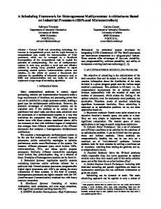
Fig. 2: ScSF schema with green color representing components developed in this work and purple representing modified and improved components.

3

Architecture and simulation process

Figure 2 shows the ScSF’s architecture around a MySQL database that stores the framework’s data and meta-data. Running experiments based on a reference system requires modeling its workload first by processing the system’s scheduling logs in the workload model engine. This model is used in the experiments to generate synthetic workloads with similar characteristics to the original ones. A simulation process starts at the description of the experimental setup in an experiment definition, including workload characteristics, scheduler configuration, and simulation time. The experiment runner processes experiment definitions and orchestrates experiments accordingly. First, it invokes the workload generator to produce a synthetic workload of similar job characteristics (size, inter arrival time) as the real ones in the reference system chosen. This workload may include specific jobs (e.g., workflows) according the the experiment definition. Next, the runner invokes the simulator that wraps Slurm to increase its execution pace and emulate the HPC system and users interacting with it. The simulator sets Slurm’s configuration according to the experiment definition and emulates the submission of the synthetic workload jobs. Slurm schedules the jobs over the virtual resources until the last workload job is submitted. At that moment, the simulation is considered completed. Completed simulations are processed by the workload analyzer. The analysis on a simulation result covers the characterization of jobs, workflows, and system. This module includes tools to compare experiments to differentiate the effects of scheduling behaviors on the workload. In the rest of this section we present the components of the framework involved in these processes. 3.1

Workload model engine

A workload model is composed of statistical data that allows creating synthetic jobs that with characteristics similar to the original ones. To create this model, first, the workload model engine extracts batch job’s variable values from Slurm or Moab scheduling logs including wait time, allocated CPU cores, requested wall clock time, actual runtime, inter-arrival time, and runtime accuruntime racy ( requestedW allClockT ime ). Jobs with missing information (e.g. start time), or

6

Gonzalo P. Rodrigo et al.

Fig. 3: Empirical distribution constructions for job variables: calculating a cumulative histogram and transforming it into a mapping table. trace type subtraces system workflow policy

”single”: regular experiment.”grouped”: experiments aggregated. list of single experiments related to this grouped one. name of system to model workload after ”period”: one workflow workflow period s. ”percent”: workflow share corehours are workflows. ”no”: no workflows. manifest list list of workflows to appear in the workload. workflow handling workflows submission in workload. ”single”: pilot job.”multi”: chained jobs”. ”manifest”: workflow-aware job start date submit time of first job valid for analysis. preload time s time to prepend to the workload for stabilization. workload duration s workload stops at start date+ workload duration s. seed string to init random number generators. Table 1: Experiment definition fields

individual rare and very large jobs that would skew the model (e.g. system test jobs) are filtered out. Next, the extracted values are used to produce the empirical distributions [15] of each job variable as illustrated in Figure 3. A normalized histogram is calculated on the source values. Then, the histogram is transformed into a cumulative histogram, i.e., each bin represents the percentage of observed values that are less or equal to the upper boundary of the bin. Finally, the cumulative histogram is transformed into a table that maps probability ranges on a value: e.g. in Figure 3, bin (10 − 20] becomes a [0.3, 0.8) probability range as its value is 80% and its left’s neighboring bin value is 30%. The probability ranges map to to the mid value of the bin range that they correspond to, e.g., 15 is the mid value of (10 − 20]. This model is then ready to produce values, e.g., a random number (0.91) is mapped on the table, obtaining 25. Each variable’s histograms is calculated with specific bin sizes adapted to its resolution. By default, the bin size for the request job’s wall clock time is one minute (Slurm’s resolution). The corresponding bin size for inter-arrival time is one second as that is the timestamp log resolution. Finally, for the job CPU core allocation, the bin size is the number of cores per node of the reference system, as in HPC systems node sharing is usually disabled. 3.2

Experiment definition

An experiment definition governs the experimental conditions in an experiment process, configuring the scheduler, workload characteristics, and experiment duration. A definition is composed by a scheduler configuration file and an experiments database entry (Table 1) that includes:

ScSF: A Scheduling Simulation Framework 1 2 3 4

7

{ " tasks " : [ { " id " : " SWide " , " cmd " : "./ W . py " , " cores " : 4 8 0 , " rtime " : 3 6 0 . 0 } , { " id " : " SLong " , " cmd " : "./ L . py " , " cores " : 4 8 , " rtime " : 1 4 4 0 . 0 , " deps " : [ " SWide " ] } ] } Fig. 4: WideLong workflow manifest in JSON format.

trace type and subtraces: The tag ”single” identifies those experiments which are meant to be run in the simulator. A workload will be generated and run through the simulator for later analysis. The experiments with trace type ”grouped” are definitions that list the experiments that are the different repetitions of the same experimental conditions in the ”subtraces” field. system model: selects which system model is to be used to produce the workload in the experiment. workflow policy: controls presence of workflows in the workload. If set to ”no”, workflows are not present. If set to ”period” a workflow is submitted periodically once every workflow period s seconds. If set to ”percentage”, workflows contribute workflow share of the workload core hours. manifest list: List of pairs (share, workflow) defining the workflows present in the workload: e.g., {(0.4 Montage.json ), (0.6 Sipht.json )} indicates that 40% of the workflows will be Montage, and 60% Sipht . The workflow field points to a JSON file specifying the structure of the workflow. Figure 4 is an example of the such file. It includes two tasks, the first running for 10 minute, allocating 480 cores (wide task); and the second running for 40 minutes, allocating 48 cores (long task).The SLong task requires SWide to be completed before it starts. workflow handling: This parameter controls the method to submit workflows. The workload generators supports workflows submitted as chained jobs (multi ), in which workflow tasks are submitted as independent jobs, expressing their relationship as job completion dependencies. Under this method, workflow tasks allocate exactly the resources they need, but intermediate job wait times might be long, increasing the turnaround time. Another approach supported is the pilot job (single), in which a workflow is submitted as a single job, allocating the maximum resource required within the workflow for its minimum possible runtime. The workflow tasks are run within the job, with no intermediate wait times, and thus, producing shorter turnaround times. However, it over-allocates resources, that are left idle at certain stages of the workflow. start date, preload time s, and workload duration s: defines the duration of the experiment workload. start date sets the submit time of the first job in the analyzed section of the workload, which will span until (start date + workload duration s). Before the main section, a workload of preload time s seconds is prepended, to cover the cold start and stabilization of the system. Random seed: this alphanumeric string is used to initialize the random generator within the workload generator. If two experiments definitions have the same parameters, including the seed, their workloads will become identical. If two experiment definitions have the same parameters, but a different seed, their workloads will become similar in overall characteristics, but different as individual jobs (i.e. repetitions of the same experiment). In general, repetitions of the

8

Gonzalo P. Rodrigo et al.

Fig. 5: Steps to run an experiment (numbers circled indicate order) taken by the experiment runner component. Once step seven is completed, the step sequence is re-started.

same experiment with different seeds are subtraces of a ”grouped” type experiment. 3.3

Experiment runner

The experiment runner is an orchestration component that controls the workload generation and scheduling simulation. It invokes the workload generator and controls through SSH a VM that contains a Slurm simulator instance. Figure 5 presents the experiment runner operations after being invoked with a hostname or IP of a Slurm simulator VM. First, the runner reboots the VM (step 0) to clear processes, memory, and reset the operative system state. Next, an experiment definition is retrieved from the database (step 1) and the workload generator produces the corresponding experiment’s workload file (step 2). This file is transferred to the VM (step 4) together with the corresponding Slurm configuration files (obtained in step 3). Then, the simulation inside the VM (step 5) is started, which will stop after the last job of the workload is submitted in the simulation plus extra time to avoid including the system termination noise in the results. The experiment runner monitors Slurm (step 6), and when it terminates, the resulting scheduler logs are extracted and inserted in the central database (step 7). Only one experiment runner can start per simulator VM, however multiple runners manage multiple VMs in parallel, which enables a simple scaling mechanism to run experiments concurrently. 3.4

Workload generation

The workload generator in ScSF produces synthetic workloads representative of real system models. The workload structure is presented in Figure 6: All workloads start with a fill phase, which includes a group of jobs meant to fill the system. The fill job phase is followed by the stabilization phase, which include 24 hours of regular jobs controlled by a job-pressure mechanism to ensure that there are enough jobs to keep the system utilized. The stabilization phase captures the cold start of the system, and it is ignored in later analysis. The next

ScSF: A Scheduling Simulation Framework

9

Fig. 6: Sections of a workload: fill, stabilization, experiment, and drain. Presented with an the associated utilization that this workload produced in the system.

stage is the experiment phase that runs for a fixed time (72 hours in the figure) and includes regular batch jobs complemented by the experiment specific jobs (in this case workflows). Although not present in the workload, after the workload is completely submitted, the simulation runs for extra time (drain period, configured in the simulator) to avoid the presence of noise from the system termination in the experiment section. In the rest of this section, we present all the mechanisms involved in detail.

Job generation: The workload generator produces synthetic workloads according to an experiment definition. The system model set in the definition is combined with a random number generator to produce synthetic batch jobs. The system model is chosen among those produced by the workload model engine (Section 3.1). Also, the random generator is initialized with the experiment definition’s seed. Finally, the workload generator also supports the inclusion of workflows according to the experiment definition (Section 3.2). The workload generator fidelity is evaluated by modeling NERSC’s Edison and comparing one year of synthetic workload with the system jobs in 2015. The characteristics of both workloads are presented in Figure 7, where the histogram and CDFs for inter arrival time, wall clock limit and allocated number of cores are almost identical. For runtime there are small differences in the histogram that barely impact the CDF.

Filling and load mechanisms: Users of a HPC system submit a job load that fills the systems and creates a backlog of jobs that induces an overall system wait time. The filling and load mechanisms steer the job generation to reproduce this phenomena. The load mechanism ensures that the size of the backlog of jobs does not change significantly. It induces a job pressure (submitted over produced work) close to a configured value, usually 1.0. Every time a new job is added to the workload, the load mechanism calculates the current job pressure t as P (t) = coreHoursSubmitted coreHoursP roduced(t) where coreHoursP roduced = t ∗ coresInT heSystem. If P (t) < 1.0 new jobs are generated and also inserted in the same submit time until P (t) ≥ 1.0. If P (t) ≥ 1.1, the submit time is kept as reference, but the job is discarded, to avoid overflowing the system. The effect of the load mechanism is observed in Figure 9, where the utilization raises to values close to one for the same workload parameters as in Figure 8.

10

Gonzalo P. Rodrigo et al.

Fig. 7: Job characteristics in a year of Edison’s real workload (darker) vs. a year of synthetic workload (lighter). Distributions are similar.

Increasing the job pressure raises system utilization but does not induce the backlog of jobs and associated overall wait time that is present in real systems. As an example, Figure 12a presents the median wait time of the jobs submitted in every minute of the experiment using the load mechanism of Figure 9. Here, the system is utilized but the jobs wait time is very short, only increasing to values of 15 minutes for larger jobs (over 96 core hours) at the end of the stabilization period (vs. the four hours intended). The fill mechanism inserts an initial job backlog equivalent to the experiment configured overall wait time. The filling jobs characteristics guarantee that they will not end at the same time or allocate too many cores. As a consequence, the scheduler is able to fill gaps left when they end. Figure 10 shows an experi-

Fig. 8: No Job pressure mechanism, No Fill: Fig. 9: Job pressure 1.0, No Fill: Low utiLow utilization due not enough work. lization due to no initial filling jobs.

Fig. 10: Job pressure 1.0, Fill with large Fig. 11: Job pressure 1.0, Fill with small jobs: initial falling spikes. jobs: Good utilization, more stable start.

ScSF: A Scheduling Simulation Framework

11

Fig. 12: Median wait time of job’s submitted in each minute. a: Job pressure 1.0, not fill mechanism, and thus no wait time baseline is present. b: Job pressure 1.0, fill mechanism configured to induce four hours of wait time baseline.

ment in which the fill job allocations are too big, their allocation is 33,516 cores (1/4 of the system CPU cores count). Every time a fill job ends (t = 8, 9, 10, and 11h), one drop in the utilization is observed because the scheduler has to fill a too large gap with small jobs. To avoid this, the filling mechanism calculates a fill job size that induces the desired overall wait time while not producing utilization drops. Fill job size calculation is based on a fixed inter-arrival time, the capacity of the system, and the desired wait time. Figure 11 shows the utilization of a workload which fill jobs are calculated following such method. They are submitted in 10 second intervals creating the soft slope in the figure. Figure 12b shows the wait time evolution for the same workload, sustained around four hours after the fill jobs are submitted. Customization: The workload generator includes classes to define user job submission patterns. Trigger classes define mechanisms to decide the insertion times pattern, such as: periodic, alarm (at one or multiple time stamps), reprogrammable alarm), or random. The job pattern is set as a fixed jobs sequence, or a weighted random selection between patterns. Once a generator is integrated it is selected by setting a special string in the workflow policy field of the experiment definition. 3.5

Slurm and the Simulator

Slurm’s version 14.3.8 was chosen as the scheduler of the framework: It is one of the most popular open-source workload managers in HPC. Also, as a real scheduler, it includes the effect and interaction of mechanisms such as priority engines, scheduling algorithms, node placement algorithms, compute nodes management, job submissions system, and scheduling accounting. Finally, Slurm includes a simulator to use it on top of an emulated version of an HPC system, submitting a trace of jobs to it, and accelerating its execution. This tool enables experimentation without requiring the use of a real HPC system. In this section, we present a brief introduction to the simulator’s structure and the improvements that we performed on it.

12

Gonzalo P. Rodrigo et al.

Fig. 13: Slurm simulator architecture. Slurm system calls are replaced to speed-up execution. Scheduling is synchronized. Job submission is emulated.

Fig. 14: Simulated time running during RPC communications delay resource de-allocation compromising backfilling’s job planning and Job B start.

Architecture: The architecture of Slurm and its simulator is presented in Figure 13. The Slurm daemons (slurmctld and slurmd) are wrapped by the emulator. Both daemons are dynamically linked by the sim func library which adds the required functions to support the acceleration of Slurm’s execution. Also, slurmd is compiled including a resource and job emulator. On the simulator side, the sim mgr controls the three core functions of the system: execution time acceleration, synchronization of the scheduling processes, and emulation of the job submission. These functions are described bellow. Time acceleration: In order to accelerate the execution time, the simulator decouples the Slurm binaries from the real system time. Slurm binaries are dynamically linked with the sim func library, replacing the time, sleep, and wait system calls. Replaced system calls use an epoch value controlled by the time controller. For example, if the time controller sets the simulated time to 1485551988, any calls to time will return 1485551988 regardless of the system time. This reduces the wait times within Slurm: e.g., if the scheduling is configured to run once every 30 simulated second, it may run once every 300 real time milliseconds. Scheduling and simulation synchronization: The original simulated time pace set by CSCS produces small speed ups for large simulated systems. However, increasing the simulated time pace triggers timing problems because of the RPC nature of Slurm daemon communications. For example, RPC under second real time latency is measured by Slurm as hundreds of simulated seconds. Increasing the simulation pace has different negative effects. First, timeouts occur triggering multiple RPC re-transmissions degrading the performance of Slurm and the simulator. Second, job timing determinism degrades. Each time a job ends, slurmd sends an RPC notification to slurmctld, and its arrival time is considered the job end time. This time is imprecise if the simulated time increases during the RPC notification propagation. As a consequence low utilization and large job (e.g. allocating 30% of the resources) starvation ocurs. Figure 14 details this effect: A large JobB is to be executed after JobA . However, JobA resources are not considered free until two sequential RPC calls are completed (end of job and epilogue), lowering the utilization as they are not producing work. The later resource liberation also disables JobB from starting but does not stop the jobs

ScSF: A Scheduling Simulation Framework

13

that programmed are to start after JobB . As the process repeats, the utilization loss accumulates and JobB is delayed indefinitely. The time controller component of the sim mgr was modified to control a synchronization crossbar among the Slurm functions that are relevant to the scheduling timing. This solves the described synchronization problems by controlling the simulation time and avoiding its increase while RPC calls are traveling between the Slurm daemons. Job submission and simulation: The job submitter component of the sim mgr emulates the submission of jobs to slurmctld following the workload trace of the simulation. Before submitting each job, it communicates the actual runtime (different from the requested one) to the resource emulator in slurmd. Slurmctld notifies slurmd of the scheduling of a job through an RPC. The emulator uses the notification arrival time and job runtime (received from sim mgr) to calculate the job end time. When the job end time is reached, the emulator forces slurmd to communicate that the job has ended to slurmctld. This process emulates the job execution and resource allocation. 3.6

Workload analyzer

ScSF includes analysis tools to extract relevant information across repetitions of the same experiment or to plot and compare results from multiple experimental conditions. Value extraction and analysis: Simulation results are processed by the workload analyzer. The jobs in the fill, stabilization, and drain phases (Figure 6) are discarded to then extract (1) for all jobs: wait time, runtime, requested runtime, user accuracy (estimating the runtime), allocated CPU cores, turnaround time, and slowdown grouped by jobs sizes. (2) for all and by type of workflow: wait time, runtime, turnaround time, stretch factor. (3) overall: median job wait time and mean utilization for each minute of the experiment. The module performs different analyses for different data types. Percentile and histograms analyze the distribution and trend of the the jobs’ and workflows’ variables. Integrated utilization (i.e., coreHoursProduced/coreHoursExecuted) measure the impact of the scheduling behavior on the system usage. Finally, customized analysis modules can be implement and added to the analysis pipeline. Repetitions and comparisons: Experiments are repeated with different random seeds to ensure that observed phenomena are not isolated occurrences. The workload analysis module analyzes all the repetitions together, merging the results to ease later analysis. Also, experiments might be grouped if they differ only in one experimental condition. The analysis module studies these groups together to analyze the effect of that experimental condition on the system. For instance, some experiments are identical except for the workflow submission

14

Gonzalo P. Rodrigo et al.

method, which affects the number of workflows that get to execute in each experiment. The module calculates compared workflow turnaround times correcting any possible results skew derived from the difference in the number of executed workflows. Result analysis and plotting: Analysis results are stored in the database to allow review of visualization using the plotter component. This component includes tools to plot histograms (Figure 7), box plots, and bar charts on the median of job’s and workflow’s variables for one or multiple experiments (Figure 17). It also includes tools to plot the per minute utilization (Figures 8 to 11) and per minute median job’s wait time in an experiment (Figures 12a and b), which allows to observe dynamic effects within the simulation. Finally, it also include tools to extract and compare utilization values from multiple experiments.

4

Scheduling simulation framework use case

In this section, we describe a use case that demonstrates the use of ScSF. The case study is to, using the simulator, implement and evaluate a workflow-aware scheduling algorithm [5]. In particular, the use case includes modeling of a real HPC system, implementing a new algorithm in the Slurm simulator, and the definition of evaluation experiments. Also, we detail a distributed deployment of ScSF and present some examples of the results to illustrate the scalability of our framework. 4.1

Tuning the model

Experiments to evaluate a scheduling algorithm require workload and system models that are representative. In this use case, NERSC’s Edison is chosen as the reference system. Its workload is modeled by processing almost four years of its jobs. Next, a Slurm configuration is defined to imitate Edison’s scheduler behavior, including: Edison’s resource definition (number of nodes and hardware configuration) FCFS, backfilling with a depth of 50 jobs once every 30s, and a multi-factor priority model that takes into account age (older-higher) and job geometry (smaller-higher). The workload tuning is completed by running a set of experiments to explore different job pressure and filling configurations to induce a stable four hour wait time baseline (observed in Edison). 4.2

Implementing a workflow scheduling algorithm in Slurm

The evaluated algorithm concerns the method to submit workflows to an HPC system. As presented in Section 3.2, workflows are run as pilot jobs (i.e., single job over-allocation resources) or chained jobs (i.e., task jobs linked by dependencies supporting long turnaround times). However, the workflow-aware scheduling

ScSF: A Scheduling Simulation Framework

15

Set Wf. Submit #Wfs. Wf. Pres. #Pres. Sim. t. #Reps #Exps Agg. Sim. t. Set0 aware/single/multi 18 Period 1 per wf. 7d 6 324 2268d Set1 aware/single/multi 6 Period 6 7d 6 648 4536d Set2 aware/single/multi 6 Share 7 7d 6 756 5292d Table 2: Summary of experiments run in ScSF.

[5] is a third method that enables per job task resource allocation, while minimizing the intermediate wait times. In this section, we present the integration of the algorithm in ScSF. The algorithm integration requires to modify Slurm’s jobs submission system, and include some actions on the job queue before and after scheduling happens. First, sbatch, Slurm’s job submission RPC, and the internal job record data structure are extended to support that jobs include a workflow manifest. This enables workflow-aware jobs to be present as pilot jobs attaching a workflow description (manifest). Second, queue transformation actions are inserted before and after FCFS and backfilling act on it. Before they act, workflow jobs are transformed into task jobs but keeping the original job priority. When the scheduling is completed, original workflow jobs are restored. As a consequence, workflow task jobs are scheduled individually, but, as they share the same priority, the workflow intermediate waits are minimized.

4.3

Creating the experiments

The workflow-aware scheduling approach is evaluated by comparing its effect on workflow turnaround time and system utilization with the pilot and chained job ones. Three versions (one per approach) of experiments are created to compare the performance of the three approaches under different conditions. Table 2 presents the three sets the experiments created. Workflows in set0, express different structure properties to study their interaction with different approaches. Set1 studies the effect of the approaches on isolated workflows and includes two synthetic workflows, plus four real (Montage, Sipht, Cybershake, FloodPlain [4]) submitted with different periods (0, 1/12h, 1/6h, 1/h, 2/h, 6/h). Set2 studies the effect of the approaches on systems increasing dominated by workflows. It includes the same workflows as set1 submitted with different workflow shares (1%, 5%, 10%, 25%, 50%, 75%, 100%). In total, they sum 1728 experiments equivalent to 33 years of simulated time. Experiments are created and stored using a Python class that is initialized with all the experiment parameters. Synthetic workflows manifest files are created manually following the framework’s manifest JSON format. Real workflow manifests are created using a workflow generator from the Pegasus project [4] that captures the characteristics of popular research workflows. ScSF includes a tool to transform the output of this generator into the expected JSON format.

16

Gonzalo P. Rodrigo et al.

Fig. 15: Schema of the distributed execution environment: VMs containing the Slurm Simulator are distributed in hosts at LBNL and UMU. Each VM is controlled by an instance of the experiment runner in the controller host at LBNL.

4.4

Running experiments in scale

1728 individual experiments that sum 33 years of simulated time are required to run in this use case. Estimating an average speedup of 10x, experiment simulation would require more than three years of real time. In order to reduce the real time required to complete this work, simulation is parallelized to increase throughput. As presented in Section 3, the minimum experiment worker unit is composed by an instance of the experiment runner component and a VM containing the Slurm simulator. As shown in Figure 15, parallelization is achieved by running multiple worker units concurrently. To configure the infrastructure, Virtualbox’s hypervisor is deployed on six compute nodes at the Lawrence Berkeley National Lab (LBNL) and 17 compute nodes at Ume˚ a University (UMU). Over them, 161 Slurm Simulator VMs are deployed. Each VM allocates two cores, four GB of RAM, and 20GB of storage. Each compute node has different configurations and thus, the number of VMs per host and their performance is not uniform, e.g., some compute nodes only host two VMs, and some host 15. All the experiment runners run in a single compute node at LBNL (Ubuntu, 12 cores x 2.8GHz, 36GB RAM). However, VMs are not exposed directly through their host NIC and, required access from the control node over sshuttle [3]: a VPN over ssh software that does not required installation in the destination host. Even if both sites are distant, the network is not a significant source of problem since the connection between UMU and LBNL traverses two high performance research networks, Nordunet (Sweden) and ESnet (EU and USA). Latency is relatively low (170-200ms), data-rate is high (firewall capped ≈100Mbits/s per TCP flow), and stability consistent. 4.5

Experimental performance

The experiments wall clock time is characterized as a function of their experimental setup to understand the factors driving simulation speed-up. Figure 16 shows the experiments median runtime of one experiment set, grouped by scheduling method, workflow type, and workflow presence. For the same simulated time, simulations run longer time under the chained job and workflow-aware approaches compared to pilot job. Also, for the chained job and aware approaches, experiments run longer time if more workflows are

ScSF: A Scheduling Simulation Framework

17

Fig. 16: Median wall clock time for a set of simulation. More complex workloads (more workflows, large workflows) present longer times. Pilot job approach presents shorter times. Simulation time is 168 hours (7 days).

present, or the workflows include more task jobs. As individual experiments are analyzed, longer runtimes, and thus smaller speed-ups, appear to be related to longer runtime of the scheduling passes because of higher numbers of jobs in the waiting queue. In summary, simulations containing numbers of jobs similar to real system workloads present median runtimes between 10 to 12 hours for 7 days (168h) of simulated time, or 15x speedup. Speed-up degrades as experiments become more complex. Speed-ups under 1 are observed for experiments whose large job count would be hard to manage for a production scheduler (e.g., Montage-75%). To conclude, the limiting factor of the simulations speed-up is the scheduling runtime, which, in this use case, depends on the number of jobs in the waiting queue. 4.6

Analyzing at scale

The analysis of the presented use case required to synthesize the results of 1278 experiments into meaningful, understandable metrics. The tools described in Section 3.6 supported this task. As an example, Figure 17 condenses the results of 324 experiments (six repetitions per experiment setting): median workflow runtime speed up (left) and value (right) observed for Cybershake, Sipht, and Montage, for different workflow shares and scheduling approaches. Results show that chained job workflows support much longer runtime in all cases, while aware and pilot jobs workflows show shorter and similar runtimes.

5

Lessons learned

The initial design goal of ScSF was readiness, not scale, and its first deployment included four worker VMs. As the number experiments and simulation time grew in the use case (33 years), the resource pool size had to be increased (161 VMs and 24 physical hosts), even expanding to resources in different locations. In this

18

Gonzalo P. Rodrigo et al.

Fig. 17: Comparison of median workflow runtime on different experimental conditions as speed-up (left), and absolute numbers (right). Data of workflows in 108 experiments.

section, we describe some of the resulting problems and what we learned from them. Loss-less experiment restart is needed: As the framework runs longer and on more nodes, the probability for node reboots becomes higher. In the months of experiments our resources required rebooting due to power cuts, hypervisor failures, VM freezes, and system updates (e.g. we had to update the whole cluster to patch the Dirty Cow exploit [1]). Unfortunately, in ScSF, rebooting a worker host means that all simulation work in its VMs is lost. Also, if the controller host is rebooted, all the experiment runners are stopped and all the simulation work of all the cluster is lost. For some of the longest experiments, the amount of work lost accounts in days of real time. The lesson learned is that experiments in ScSF should support graceful pause and restart so resource reboots do not imply loss of work. This would be provided by a control mechanism to pause-restart worker VMs. Also, the experiment runner functionality should be hosted in the worker VM to be paused with the VM, unaffected by any reboot. Loaded systems network fail: Surges of experiment failures appeared occasionally: Multiple VMs would become temporarily un-responsive to ssh connections when their hypervisor was heavily loaded. Subsequently, the experiment runner would fail to connect to the VM, and the experiment was considered failed. The lesson learned is that saturated resources are unreliable. All runnerVM communications were hardened, adding re-trials, which reduced greatly the fail rate. Monitoring is important: Many types of failure impact on experiments, such as simulator or Slurm bugs, communication problems, resource saturation in the VMs, or hypervisor configuration issues. Failures are expected, but ScSF lacked the tools and information to quickly diagnose the cause of the problems. The lesson learned is that monitoring should register metadata that allows quick diagnosis of problems. As a consequence, details level in experiment logs was increased and a mechanism to retrieve Slurm crash debug files was added. The system is as weak as its weakest link: All ScSF’s data and metadata is stored in a MySQL database hosted in the controller host. In a first experiment run, at 80% of completed experiments the hard disk containing the database

ScSF: A Scheduling Simulation Framework

19

crashed, and all the experimental data was lost. Two months of real time were lost and an article submission deadline was missed. Currently, data is subject to periodic backups and the database is replicated.

6

Conclusions

We present ScSF, a scheduling simulation framework that provides tools to support all the steps of the scheduling research cycle - modeling, generation, simulation, and result analysis. ScSF is scalable, it is deployed over distributed resources to run and manage multiple concurrent simulations and provides tools to synthesize results over large experiment sets. The framework produces representative results by relying on Slurm, which captures the behavior of the real system schedulers. ScSF is also modular and might be extended by researchers to generate customized workloads or calculate new analysis metrics over the results. Finally, we improved the Slurm simulator which now achieves up to 15x simulate over real time speed-ups while preserving its determinism and experiment repeatability, This work provides a foundation for future scheduling research. ScSF will be liberated as open source, enabling scheduling scientists to concentrate their effort on designing scheduling techniques and evaluating them in the framework. Also, we share the experience of using ScSF to design our own scheduling algorithm and evaluating it through the simulation of a large experiment set. This experience shows that the framework is capable of simulating 33 years of real systems time in less than two months over a small distributed infrastructure. Also, it constitutes a guide for future users of the framework. Finally, our experiences building ScSF and running it in scale might be of use of researchers who are building similar systems.

7

Acknowledgments

This material is based upon work supported by the U.S. Department of Energy, Office of Science, Office of Advanced Scientific Computing Research (ASCR). The National Energy Research Scientific Computing Center, a DOE Office of Science User Facility, is supported by the Office of Science of the U.S. Department of Energy under Contract No. DE-AC02-05CH11231. Financial support has been provided in part by the Swedish Government’s strategic effort eSSENCE and the Swedish Research Council (VR) under contract number C0590801 (Cloud Control). Special thanks to Stephen Trofinoff and Massimo Benini from the Swiss National Supercomputing Centre, who shared with us the code base of their Slurm Simulator. Also, we would like to thank the members of the DST department at LBNL and the distributed systems group at Ume˚ a University who administrated or gave-up the compute nodes supporting the use case.

References 1. Dirty cow (January 2017), https://dirtycow.ninja/

20

Gonzalo P. Rodrigo et al.

2. SchedMD (January 2017), https://www.schedmd.com/ 3. shuttle (January 2017), https://github.com/apenwarr/sshuttle 4. Workflowgenerator (1 2017), https://confluence.pegasus.isi.edu/display/ pegasus/WorkflowGenerator ¨ 5. Alvarez, G.P.R., Elmroth, E., Ostberg, P.O., Ramakrishnan, L.: Enabling workflow aware scheduling on hpc systems. In: Under review for HDPC 2017 ¨ 6. Alvarez, G.P.R., Ostberg, P.O., Elmroth, E., Antypas, K., Gerber, R., Ramakrishnan, L.: Towards understanding job heterogeneity in hpc: A nersc case study. In: 2016 16th IEEE/ACM International Symposium on Cluster, Cloud and Grid Computing (CCGrid). pp. 521–526. IEEE (2016) 7. Declerck, T.M., Sakrejda, I.: External Torque/Moab on an XC30 and Fairshare. Tech. rep., NERSC, Lawrence Berkeley National Lab (2013) 8. Feitelson, D.: Parallel workloads archive 71(86), 337–360 (2007), http://www.cs. huji.ac.il/labs/parallel/workload 9. Feitelson, D.G.: Workload modeling for computer systems performance evaluation. Cambridge University Press (2015) 10. Feitelson, D.G., Tsafrir, D.: Workload sanitation for performance evaluation. In: 2006 IEEE international symposium on Performance analysis of systems and software. pp. 221–230. IEEE (2006) 11. IBM: Platform computing lsf. http://www-03.ibm.com/systems/ technicalcomputing/platformcomputing/products/lsf/sessionscheduler. html (January 2014) 12. Jackson, D., Snell, Q., Clement, M.: Core algorithms of the maui scheduler. In: Job Scheduling Strategies for Parallel Processing. pp. 87–102. Springer (2001) 13. Kannan, S., Mayes, P., Roberts, M., Brelsford, D., Skovira, J.: Workload Management with LoadLeveler. IBM Corp. (2001) 14. Klus´ aˇcek, D., Rudov´ a, H.: Alea 2 – job scheduling simulator. In: Proceedings of the 3rd International ICST Conference on Simulation Tools and Techniques (SIMUTools 2010). ICST (2010) 15. Lublin, U., Feitelson, D.G.: The workload on parallel supercomputers: modeling the characteristics of rigid jobs. Journal of Parallel and Distributed Computing 63(11), 1105–1122 (2003) 16. Lucero, A.: Simulation of batch scheduling using real production-ready software tools. Proceedings of the 5th IBERGRID (2011) ¨ 17. Rodrigo, G., Ostberg, P.O., Elmroth, E., Antypass, K., Gerber, R., Ramakrishnan, L.: HPC system lifetime story: Workload characterization and evolutionary analyses on NERSC systems. In: The 24th International ACM Symposium on High-Performance Distributed Computing (HPDC) (2015) 18. Schwiegelshohn, U.: How to design a job scheduling algorithm. In: Workshop on Job Scheduling Strategies for Parallel Processing. pp. 147–167. Springer (2014) 19. Stephen Trofinoff, M.B.: Using and Modifying the BSC Slurm Workload Simulator. In: Slurm User Group (2015) 20. Yoo, A., Jette, M., Grondona, M.: SLURM: Simple Linux Utility for Resource Management. In: Feitelson, D., Rudolph, L., Schwiegelshohn, U. (eds.) Job Scheduling Strategies for Parallel Processing, Lecture Notes in Computer Science, vol. 2862, pp. 44–60. Springer Berlin / Heidelberg (2003) 21. Zakay, N., Feitelson, D.G.: Preserving user behavior characteristics in trace-based simulation of parallel job scheduling. In: IEEE 22nd International Symposium on Modelling, Analysis & Simulation of Computer and Telecommunication Systems (MASCOTS), 2014. pp. 51–60. IEEE (2014)