Color Image Segmentation with Genetic Algorithm for In-Field Weed

PUBLICATION VERSION

Color Image Segmentation with Genetic Algorithm for In-Field Weed Sensing L. Tang, L. F. Tian, B.L. Steward

ABSTRACT This study was undertaken to develop machine vision-based weed detection technology for outdoor natural lighting conditions. Supervised color image segmentation using a binary-coded genetic algorithm (GA) identifying a region in Hue-Saturation-Intensity (HSI) color space (GAHSI) for outdoor field weed sensing was successfully implemented. Images from two extreme intensity lighting conditions, those under sunny and cloudy sky conditions, were mosaicked to explore the possibility of using GAHSI to locate a plant region in color space when these two extremes were presented simultaneously. The GAHSI result provided evidence for the existence and separability of such a region. In the experiment, GAHSI performance was measured by comparing the GAHSIsegmented image with a corresponding hand-segmented reference image. When compared with cluster analysis-based segmentation results, the GAHSI achieved equivalent performance.

Keywords Genetic algorithm, Weed sensing, Color image segmentation, Lighting condition. Article Notes Article was submitted for publication in April 1999; reviewed and approved for publication by the Information & Electrical Technologies Div. Of ASAE in January 2000. The use of trade names is only meant to provide specific information to the reader and does not constitute endorsement by the University of Illinois. The authors are Lie Tang, ASAE Student Member, Graduate Student, Lei F. Tian, ASAE Member, Assistant Professor, Department of Agricultural Engineering, University of Illinois at Urbana-Champaign, Urbana, IL; and. Brian L. Steward, ASAE member, Assistant Professor, Agricultural and Biosystems Engineering Department, Iowa State University, Ames, IA 50011. Corresponding Author: Lei F. Tian, University of Illinois, 1304 W. Pennsylvania Ave., Urbana, IL 61801; tel: (217) 333-7534; fax: (217) 244-0323; e-mail: [email protected].

1

INTRODUCTION The application of machine vision for weed sensing is promising because it utilizes not only spectral information, but also spatial and textural information. One of the challenges in the development of robust weed sensing technology is the variability associated with outdoor lighting conditions. Tian and Slaughter (1998) investigated the application of a machine vision system in an crop field and found that direct sunlight causes substantial intensity differences within the images from the low intensity of shadows to the high intensity of shiny leaf surface reflections. Daylight varies greatly in intensity as well as in color temperature (Wyszecki and Stiles, 1982; Henderson, 1977).

In the case of in-field machine vision-based weed sensing, it is essential to correctly divide images into regions which are plants (weeds or crop) and background (soil, rocks and residue). Image segmentation is an important and perhaps the most difficult image processing task. Segmentation refers to subdividing an image into regions exhibiting "similar" characteristics. Subsequent image interpretation tasks, such as feature extraction and object recognition, rely on the quality of the segmentation results. The difficulty arises when the segmentation performance needs to be adapted to the changes in image quality. Image quality is usually affected by variations in environmental conditions, imaging devices and time of day. Despite the large number of segmentation techniques presently available, no general methods have been found to perform adequately across a diverse set of imagery under variable lighting conditions.

Genetic algorithms (GA) are a family of adaptive search methods that are modeled after the genetic evolutionary process. An attractive feature of GAs is their high efficiency dealing with difficult combinatorial search problems without being stuck in local extrema through their parallel exploration of the search space. Therefore, they have become powerful alternatives to conventional optimization methods (Goldberg, 1989a). GAs have been used for image segmentation in the past. Andrey and Tarroux (1994) used a distributed GA for unsupervised image segmentation. The GA was applied to intensively modify a labeling function. Fitness evaluation was based on region homogeneity and specificity. Bhanu et al. (1995) conducted research on adaptive image segmentation using genetic and hybrid search methods. A multi-objective optimization GA was

2

used as a machine learning component in a feedback loop to select an input parameter set for a Phoenix algorithm, which is a recursive region splitting technique that contains seventeen different control parameters. Five different segmentation quality measures were incorporated to determine overall fitness for a particular parameter set. Andrey and Tarroux (1998) used selectionist relaxation for unsupervised segmentation of Markov random field modeled textured images. The transformation of an input image into a segmented output image was computed by a population of units that iteratively evolves through a distributed GA, where each unit was an association between a candidate feature vector and a label. However, none of the three above studies utilized GA-based color image segmentation. Their efforts were primarily focused on unsupervised and adaptive considerations, and their objective was to classify as many regions as possible based on their specific criteria.

Until now, however, most of the machine vision weed sensing research has been done under controlled lighting conditions rather than natural variable lighting conditions. Woebbecke et al. (1995) studied the use of color indices for weed segmentation with shaded and unshaded plant surfaces presented in images. They determined that the best segmentation occurred with the modified hue and 2g-r-b (excessive green) contrast index, where r, g and b were normalized R, G and B. However, leaf “hole” pixels were created due to conversion of the images from 24-bit to 8-bit, i.e., 3 dimensional image information was reduced to 1 dimension before segmentation. Some vegetation image segmentation methods have been based on cluster analysis (Tian et al, 1997; Steward and Tian, 1998). Cluster analysis-based segmentation is sensitive to lighting conditions, choice of cluster seeds, and number of clusters. For instance, if the composition of different image portions from different lighting conditions changed, then the clustering result would be different. Thus, it is difficult to create a universal cluster map to robustly sense weed under variable lighting conditions. In the cluster analysis-based approaches, cluster analysis is first used to divide the image data according to similarities in color. Then after plant regions are labeled as such by visual inspection, a Bayes classifier is trained and used to generate a LUT which is employed during real-time segmentation. For real-time weed sensing, a LUT can use computer memory to trade for speed. However, as Fu and Mui (1981) pointed out, one of the shortcomings of the clustering process is that it does not take into account spatial interactions among neighboring pixels, thus results in a lower segmentation quality.

3

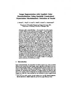
The objective of this study was to explore the possibility of detecting – through the use of a GA – a relatively stable color region in HSI color space to segment vegetation under two extreme outdoor field lighting conditions resulting from cloudy and sunny sky conditions. This color region could be then used to distinguish weeds under a large variety of lighting conditions. MATERIALS In this research, a 3-CCD (Sony Model No. XC-003) color video camera was employed to capture the images. The camera was mounted at a height of 3.35 m (11 ft) on a custom-made camera boom for a Patriot XL sprayer (Tyler Industries, Benson, MN). The Y/C output of the camera was routed to an Imagenation (Beaverton, OR) PXC200 color frame grabber housed in a Pentium-based portable computer. The frame grabber had a resolution of 640 by 486 pixels. Each pixel corresponded to an area of approximately 0.002 by 0.002 m. Images were taken while the sprayer was moving with a forward travel speed of 0.6 km/hour (0.4 miles/hour) to minimize motion effects. The soybeans were approximately 0.13 m. (5 in.) high at the time the images were taken. The first set of images was taken in the morning of June 29, 1998 under cloudy conditions, and the second set was taken in the afternoon of the same day under sunny conditions (Steward and Tian, 1998). To form a mosaicked image, four images were selected from these image set with two images from sunny lighting conditions and the other two images from cloudy lighting conditions. The size of the mosaicked image was 640x800 pixels, which comprised four 640x200 pixel portions. Each portion was clipped from one of the selected images. A part of mosaicked image was provided to show it was constructed (Figure 1). The left-hand portion was from an image acquired under sunny lighting condition with low-vegetation density and the right-hand portion was from an image acquired under cloudy lighting condition with high-vegetation density. The purpose of mosaicking together images of different lighting condition was to determine if the GA could tolerate the lighting variation and locate a color region in HSI space to use for segmenting plants from background. The different vegetation density provided a larger range of color variations so that the mosaicked image better represented the vegetation color features in typical outdoor field conditions. Manual segmentation was performed by humans painting the plant pixels in the images with a common color. This was accomplished with a commercial photo/paint software. The handsegmented images of mosaicked image and of those four selected images with their original full 4

frame size 640 x 486were used as reference images. Meanwhile, the same set of four selected unsegmented-images was used as test images to evaluate GAHSI segmentation results. DATA TRANSFORMATION Intensity dominates the scatter in the pixel data in RGB (Red, Green, and Blue) space with data points forming cigar-shaped regions along the intensity axis (Figure 2). This type of distribution makes simple min-max boundary type thresholding methods unfeasible. Moreover, non-normalized RGB coordinates could be greatly varied by imaging conditions (Tarbell and Reid, 1991). Normalized RGB coordinates, i.e., chromaticity coordinates form the color triangle, which defines the color components (hue and saturation) of the HSI model. As Gonzalez and Woods (1992) indicated, hue, saturation, and intensity are general characteristics used to distinguish one color from another. Hue represents the dominant wavelength in a mixture of light waves and thus is the dominant character. Saturation is the relative purity or the amount of white light mixed with a hue; hence, pure spectrum colors are fully saturated. Hue and saturation considered together is referred to as chromaticity; and therefore, a color may be characterized by its intensity and chromaticity. The HSI model decouples the intensity component from the color information, and the hue and saturation components related to the way in which human beings perceive color. Thus, the HSI model is an ideal tool for developing image processing algorithms based on some of the color sensing properties of the human visual system. The HSI model is defined by a transformation of RGB color component as:   [( R − G ) + ( R − B)] / 2  H = cos −1  2 1/ 2   [(R − G ) + ( R − B)(G − B)]  3 S = 1− [min( R, G , B)] ( R + G + B) 1 I = ( R + G + B) 3

(1) (2) (3)

A disadvantage of the HSI color system is that the transformations of hue, saturation and normalized color are all ill-conditioned (Kender, 1976). They have a singularity at the origin of R=G=B=0, and hue is also undefined along the R=G=B intensity axis. These transforms are unstable near their singularities. Thus sensor noise or minor reflectance variations lead to instabilities in these transformations. Moreover, with the spurious modes and gaps existing in their

5

digitized distributions due to central normalizing division, segmentation techniques of edge detection, clustering, region splitting and growing will be deeply affected. Although there is no way of eliminating those problems, the results do imply higher dimensional segmentation methods. Therefore, segmentation methods based on HSI 3-D space theoretically tend to have better performance than single dimension color indices or normalized color-only segmentation methods.

To simplify the thresholding segmentation method, the distribution in HSI space was examined. In this research, when all three components of HSI were normalized to 0-255 with hue and saturation being 0 at their singularity (Figure 3), the distribution extended across the whole space. We surmised that there existed a cuboid region, which defined all plant pixels, because plant pixels should be "green" with varying saturation and intensity levels. However, background should be the region of "gray" pixels, consisting of soil, rock and residue. Therefore, because a “plant” region could be defined in HSI space by planes, the image data was transformed from RGB into HSI space by using equations (1-3) before the implementation of the GAHSI algorithm

ALGORITHM DESIGN In order to locate the color region in HSI space to identify all plant pixels, the total search space was defined as a matrix of six variables, which are the lower and upper boundaries of hue, saturation, and intensity. Each boundary pair has 256 x 256 combinations. This will lead to 2566 = 2.8x1014 possible boundary combinations. Thus, an efficient searching algorithm is important to solve this problem. Furthermore, the algorithm must be able to locate the global optima without being trapped by local optima. GAs are a parallel and global optimization methods. The inherent power of GAs lies in their ability to exploit accumulating information about an initially unknown domain in a highly efficient manner. Therefore, GA was selected to design a search engine in this research. GA Components and Operators Chromosome A 48-bit binary string, or a chromosome, represented “plant” region boundaries in HSI space. Each boundary parameter was assigned a byte-long fixed location in the chromosome. The relative locations of parameters are important because of how genetic algorithms choose "better"

6

combinations of parameters (Goldberg, 1989a). Features, which are likely to interact to form "building blocks", are optimally positioned adjacent to each other so that successful combinations are not easily broken up during the crossover operations. Based on the knowledge of the definition of HSI color space and the weed sensing objective, the string was organized with the upper hue boundary as the first byte in the chromosome followed by the lower hue boundary since hue is the most salient color feature. The next two bytes were the upper and lower saturation boundaries. The intensity boundaries were the last two bytes since intensity is independent of color and therefore of less importance (Table 1). Each of the three pairs of HSI upper and lower boundaries are in adjacent positions because intuitively they should be so connected to form "building blocks". Population Size The basic elements of a GA are called knowledge structures or individuals. A collection of individuals is referred to as a population. Goldberg's (1989b) rule of thumb calls for a population size approximately equal to the chromosome length. For our application with a chromosome length of 48 bits, a population size of 48 was used to generate final segmentation boundaries. Selection The expected number of times an individual is selected for recombination is proportional to its fitness relative to the rest of the population. Local tournament selection without replacement with a size of four was implemented in the GAHSI algorithm. Local tournament selection, which selects the individual with the highest fitness out of randomly picked individuals, was chosen over roulette wheel selection because it could cause premature problems at earlier stages. Crossover and Mutation Crossover and mutation determine the genetic makeup of offspring from the genetic material of the parents. A single point crossover between the selected chromosomes was utilized to generate a new population for each generation. De Jong (1975) showed that good GA performance requires a high crossover probability. Thus for the GAHSI, a crossover probability of 0.8 was adopted. Mutation provides for occasional disturbances in the crossover operation by inverting one or more genetic elements during reproduction. Goldberg (1989a) recommended a mutation rate inversely proportional to the population size, which would result in a rate of 0.02 for this application. However, since tournament selection tends to encourage convergence of the GA, a higher mutation rate was necessary. Therefore, a mutation rate of 0.03 was used in this application.

7

Constraints All upper boundaries must be larger than their corresponding lower boundaries. The processes of crossover and mutation, however, will cause these boundary constraints to be violated. A simple correction was implemented to bring the upper boundary value back to ten greater than lower boundary value when a violation was detected. This was done because the lower boundaries have more significant effects on segmentation. Function evaluation Segmentation performance measures (PMs) were applied for function evaluation. The two PMs used were object sensitivity (SenO) and background sensitivity (SenB) (Steward and Tian, 1998). SenO is the ratio of correctly segmented plant pixels in the test image to the total number of plant pixels in the reference image. SenB is the ratio of the number of correctly segmented background pixels in the test image to the total number of background pixels in the reference image (Figure 4). SenO =

Cp Cp + IB

(4)

SenB =

CB CB + I p

(5)

where:

Cp=P-IB=number of pixels correctly classified as plants in the test image with respect to the reference image. P=total number of plant pixels in the reference image. IB=number of pixels classified as plants in reference image, but as background in the test image. IP=number of pixels classified as background in reference image, but as plants in the test image. CB=B-IP=number of pixels correctly classified as background in the test image with respect to the reference image. B=total number of background pixels in the reference image.

When fitness was established as the average of SenO and SenB, it was difficult to reduce the amount of noise in the background observed after segmentation. Since the difference between the number of object and background pixels can be quite different and varying from image to image, a biased fitness, which was a weighted average of SenO and SenB by their corresponding pixel ratio

8

in the image, was used. The definitions of equally weighted fitness (FE) and biased fitness (FB) were: FE = 0.5*SenB+0.5*SenO

(6)

FB = ORatio*SenB + (1-ORatio)*SenO

(7)

Where ORatio was the ratio of the object pixel number to the total pixel number in reference image. The ORatio was 0.2384 in the mosaicked image. Stopping Criteria The GAHSI stopped when one of three conditions was satisfied. First, the process terminated if a utopia parameter set, which was the best fitness value above a predefined threshold of acceptance, was located. The threshold for acceptable segmentation in this research was set at 99% with respect to hand-segment generated reference images. Second, the process terminated if the best fitness of the populations failed to improve for five consecutive generations. Third, the process stopped if the generation number was greater than 100. When any one of these conditions was met, the overall best-fitted chromosome string was decoded as the boundaries in HSI color space of the “plant” region.

GAHSI EVALUATION METHOD To measure segmentation performance of the GAHSI generated color space division, the same set of images used by Steward and Tian (1998) were segmented. Performance measures used for their research and described above were calculated and compared with those reported in their work on clustering and color transformation-based image segmentation research. In their research, cloudy and sunny images were processed separately by four clustering and color transformationsbased algorithms. There were two type of GAHSI-based segmentation results. The results obtained when segmenting each image with its self-extracted boundaries using GAHSI were given the label GAHSI Pro. Label GAHSI Test meant that the results obtained when each image was segmented using boundaries extracted from the mosaicked image using GAHSI. Analysis of variance was used to determine if differences in segmentation performance existed across the different segmentation algorithms. Segmentation methods were grouped according to mean performance measures using Duncan’s multiple range test.

9

RESULTS AND DISCUSSION During the experiments, GA parameters and operators were adjusted to achieve a higher fitness value. With the same setup of crossover and mutation probabilities, population sizes of 100, 150, 200, and 250 were used. Fitness of 0.9003 was the best value achieved with FB function for all population sizes under 100 generations. There was no substantial improvement of the best fitness when increasing the population size. Extreme probability values (1 and 0) of crossover were tested and no final improvement of best fitness was observed. The GAHSI was still able to effect the best fitness value when extinguishing crossover, but the convergence speed was reduced. Qi and Palmieri (1995) proved that crossover explores new features of the solution space without increasing the variance of each individual coordinate. Crossover represents a bounded stochastic search scheme. The desire for improvement after the GA reached a near optimal stage, led the authors to put some efforts on adaptively adjusting the mutation rate. A genetic search has its own built-in hill climber (mutation plus selection), and thus HC-easy problems can be solved (Goldberg, 1991). When a method of turning off crossover after 20 generations was tested, only a slight improvement was obtained. It was also not a surprise because only 1 point crossover was implemented. The crossover points were much smaller than the dimension of objective function, so the effect of crossover was expected to be small. Back (1993) declared that, as long as fitness is a unimodal pseudoboolean function, a mutation rate p=1/L (L is the chromosome length) is the best choice. For multi-modal cases, a mutation rate different from 1/L may be worthwhile in order to overcome local optima. The fitness definition in this research was the combination of SenO and SenB; intuitively it could be taken as a unimodal fitness function, so mutation rate close to 0.02 should be maintained. Back also pointed out that whenever the objective function is unimodal, Gray code assures unimodality of the fitness function and therefore should be the best choice. Gray code itself represents adjacent integers by bit strings of Hamming distance one, thus that fine-tuning of near optimal solutions will be simplified by Gray code. Moreover, only a simple GA was used in the application. There is potential that an advanced GA model (messy GA) may further improve the performance of GAHSI. One messy GA method is to use "knowledge-augmented operators" for crossover. For example, multi-point crossover at boundary edges may lead to a better performance of GAHSI.

When comparing the results of the GAHSI using FE with those when FB was used, it was

10

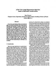
observed that FB slightly raised the lower boundaries for each HSI component (Table 2). This result was expected since FB had a higher weight on the background sensitivity which led the GA to ignore the low hue, saturation and intensity but greenish noise pixels presented around cracks in the soil. From the convergence performance curves of FB, it was observed that the near maximum fitness was quickly achieved before 10 generations (Figure 5).

The three boundaries, which had the most significant effect on segmentation performance, were the lower hue, saturation, and intensity boundaries. For population sizes of 48, 100, 150, 200, 250, GAHSI achieved the same values of these three important boundaries under 100 generation. Roulette wheel selection and tournament selection were compared in the experiment. To locate an equivalent observed optima, roulette wheel selection ran up to generation 9593, but tournament selection achieved it in less than 100 generations.

When viewing segmented images after applying the results of the GAHSI from mosaicked image, it was observed that cracks in the soil, which were darker than the surrounding soil, were often segmented as plant regions (Figure 6). This was mainly due to the non-linear mapping which took place in the RGB to HSI transformation, and the inherent instability near their singularities. This effect could be attributed to color sensor noise as well. The overall segmentation results were good in both sunny and cloudy image portions. When the image segmented by using GAHSI was compared with the reference image (Figure 6), the GAHSI apparently eliminated a lot of noise due to questionable hand segmentation. The segmentation process in HSI domain clearly showed that the GAHSI found those greenish plant hue pixels within a certain saturation and intensity range (Figure 7). The algorithm took off a certain amount of pixels in low saturation and intensity region, which was impressive, considering the transformation instability issues near its singularity. This result implies that there exists a region in HSI color space where the majority of the plant pixels exist regardless of the variation in lighting conditions. GA can easily locate this region as long as it is provided with a small sample of reference image, which is not necessarily hand-segmented very accurately. This segmentation scheme has advantages over other segmentation methods of clustering, edge detection, region growing and splitting because it is a global optimization process rather than a local information driven method, which could be more sensitive to the problems illposed in transformation, sensor noise, and imaging conditions.

11

Analysis of variance revealed that there was no significant difference for the means of SenO, SenB and Sum (Sum = SenO + SenB) variables across GAHSI Pro, GAHSI Test and ISO treatments (p=0.05) (Table 3). This result implied that application of the GAHSI algorithm on the mosaicked image provided a viable approach to resolve cloudy and sunny lighting variations. For the means of SenO and Sum variables, there was no significant difference across all six treatments with the exception of the EGRBI 1. From the results of the sum of SenO and SenB and the mean of this sum of four test images when compared with hand-segmented reference images, the variation of these sensitivity values along different segmentation schemes was illustrated. The valley only happened at EGRBI 1 (Figure 8). Based on these statistical results, we concluded that GAHSI algorithm achieved an equivalent segmentation performance as achieved by the methods based on cluster analysis.

Hand-segmentation is time consuming and tedious with questionable quality. It is also obvious that the human uses spatial as well as spectral information in the segmentation process resulting in a reference that was developed with more information than computer-based image segmentation, which is based on color information alone. The above factors could explain why GAHSI could not reach closely to 100% fitness. However, spatial information was incorporated into the hand-segmented reference image and GA used this image as the optimization target. The resulting advantage was that spatial information was used through GAHSI segmentation process, which would imply an improvement of segmentation quality. When we made a mosaic image with images under different lighting conditions combined together as reference image, GAHSI could locate a correct region to cover the plant color space. Goldberg (1989a) pointed out that “in some cases GAs prefer a noisy and crude function evaluation, which in turn permits resources to be used for exploring (even approximately) other points in the search space.” This implies that using common image processing tools could generate a reference image. A visually "good" reference image could guide the GAHSI in locating an optimal boundary in threedimensional color space. Certainly, a better reference image will allow the algorithm refine the boundary more accurately. A better approach of generating reference images is to use a segmentation algorithm which incorporates both spatial and color information, such as the segmentation model proposed by Benlloch and Rodas (1998).

12

CONCLUSIONS The GA-based segmentation scheme described in this paper is a novel and simple approach to robustly segment an outdoor field image into plant and background regions under variable lighting conditions. The performance analysis of the GAHSI revealed that, for machine vision-based weed sensing in variable lighting conditions, the genetic algorithm-based, supervised color image segmentation in HSI color space was shown to be an effective approach. The GAHSI obtained an equivalent segmentation performance to that obtained by applying cluster analysis to images acquired under specific lighting conditions. The results of applying a GA to detect a region in HSI space for plant segmentation has shown promise and could overcome the effects of variable outdoor lighting conditions with an acceptable error range. To further improve segmentation robustness, different imaging devices and color transformations as well as GA codings and operators need to be investigated in future research.

ACKNOWLEDGEMENTS This research was supported by the Illinois Council on Food and Agricultural Research (CFAR). Project No. 99I-112-3.

REFERENCES Andrey, P. and P. Tarroux. 1994. Unsupervised image segmentation using a distributed genetic algorithm. Pattern Recognition 27(5):659-673. Andrey, P. and P. Tarroux. 1998. Unsupervised segmentation of Markov random field modeled textured images using selectionist relaxation. IEEE Transactions on Pattern Analysis and Machine Intelligence 20(3):252-262. Back, T. 1993. Optimal mutation rates in genetic search. In Proceedings of the Fifth International Conference on Genetic Algorithms, 2-8. San Mateo, California: Morgan Kaufmann Publishers. Benlloch, J. and A. Rodas. 1998. Dynamic model to detect weeds in cereals under actual fields conditions. In Proc. SPIE 3543, Precision Agriculture and Biological Quality, eds. J. A.

13

DeShazer and G. E. Meyer, 302-310. Bellingham, Wash.:SPIE. Bhanu, B. ,S. Lee and S. Das. 1995. Adaptive image segmentation using genetic and hybrid search method. IEEE Transactions on Aerospace and Electronic Systems 31(4):1268-1290. De Jong, K.A. 1975. Analysis of the behavior of a class of genetic adaptive systems. Ph.D. thesis, Department of Computer and Communication Science, Univ. of Michigan. Fu, K.S. and J.K. Mui. 1981. A survey on image segmentation. Pattern Recognition 13:3-16. Goldberg, D.E. 1989a. Genetic algorithms in search, optimization and machine learning. Mass.: Addison-Wesley Publishing Company, Inc. Goldberg, D.E. 1989b. Sizing populations for serial and parallel genetic algorithms. In Proceedings of the Third International Conference on Genetic Algorithms, 70-79. San Mateo, Calif.: Morgan Kaufmann Publishers. Goldberg, D.E. 1991. Real-coded genetic algorithms, virtual alphabets, and blocking. Complex System 5:139-167. Gonzalez, R.C. and R.E. Woods. 1992. Digital Image Processing. Mass.: Addison-Wesley Publishing Company, Inc. Henderson, S.T. 1977. Daylight and Its Spectrum. New York, NY: John Wiley & Sons. Kender, J. 1976. Saturation, hue, and normalized color: calculation, digitization effects, and use. Technical Report. Pittsburgh, Pa.: Carnegie-Mellon Univ., Computer Science Department. Qi, X. and F. Palmieri. 1995. The diversification role of crossover in the genetic algorithms. In Proceedings of the Fifth International Conference on Genetic Algorithms, 132-137. San Mateo, Calif.: Morgan Kaufmann Publishers. Steward, B.L. and L. F. Tian. 1998. Real-time weed detection in outdoor field conditions. In Proc. SPIE 3543, Precision Agriculture and Biological Quality, eds. J. A. DeShazer and G. E. Meyer, 266-278. Bellingham, Wash.:SPIE. Tarbell, K.A. and J.F. Reid. 1991. A computer vision system for characterizing corn growth and development. Transactions of the ASAE 34(5):2245-2255. Tian, L and D.C. Slaughter. 1998. Environmentally adaptive segmentation algorithm for outdoor image segmentation. Computers and Electronics in Agriculture 21:153-168. Tian, L., D.C. Slaughter and R.F. Norris. 1997. Outdoor field machine vision identification of tomato seedlings for automated weed control. Transactions of the ASAE 40(6):1761-1768. Woebbecke, D.M., G.E. Meyer, K.Von Bargen and D.A. Mortensen. 1995. Color indices for

14

weed identification under various soil, residue, and lighting conditions. Transactions of the ASAE 38(1):259-269. Wyszecki, G. and W. S. Stiles. 1982. Color Science: Concepts and Methods, Quantitative Data and Formulae, 4-11. New York, NY: John Wiley & Sons.

15

Figure 1. A portion of mosaicked image

Figure 2. Mosaicked image pixel distribution in RGB color space

Figure 3. Mosaicked image pixel distribution in HSI color space

Figure 4. Venn diagram showing the pixel sets as segmented in the reference image and test image respectively. P and B are the sets of plant and background pixels in the reference image respectively. Cp is the set of correctly segmented plant pixels in the test image. Ip and Ib are the sets of pixels incorrectly segmented as plant and background respectively.

16

Table 1. Structure of chromosome string Byte 2

Byte 3

Byte 4

Byte 5

Byte 6

Hue-

Hue-

Saturation-

Saturation-

Intensity-

Intensity-

High

Low

High

Low

High

Low

Sensitivity and Fitness

Byte 1

1 0.95 0.9 0.85 0.8 0.75 0.7 0.65 0.6 0.55 0.5

SenO SenB Max Avg 0

10

20

30

Generation

Figure 5. Convergence of GAHSI with FB. Max: Maximum fitness in current generation; Avg: Average fitness in current generation . The overall maximum fitness was achieved at generation 33.

17

A

B

C

D

E

F

Figure 6. A: Original image. B: Hand-segmented reference image. C: GAHSI segmentation with FE. D: GAHSI segmentation with FB. E: Image D after one run “opening” filtering. F: Difference image of B and E.

18

Figure 7. Image pixel distribution in HSI space. Left: Plots for original image; Middle: Plots for hand-segmented plant objects; Right: Plots for GAHSI-segmented plant objects. Upper row plots: Polar plots of hue and saturation. Hue is plotted as angle ranging from 0 to 360 degree and saturation is plotted as distance ranging form 0 to 1; Bottom row plots: Plots of projection on saturation and intensity plane. 2 1.9 1.8 1.7 1.6 1.5 1.4 1.3 1.2 1.1 1

cld1 cld3 sun1 sun4

GAHSI Pro

GAHSI Test

ISO

NC

EGRBI 1 EGRBI 2

Mea n

Figure 8. Comparison of the sum of object sensitivity and background sensitivity with GAHSI to clustering segmentation algorithms on four images. GAHSI Pro: Segmentation using GAHSI algorithm; GAHSI Test: Segmentation using boundaries extracted by GAHSI algorithm from the mosaicked image; ISO: ISODATA; NC: EASA after normalized color transformation; EGRBI 1: EASA after EGRBI transformation with 1 plant cluster; EGRBI 2: EASA after EGRBI transformation with 2 plant clusters 19

Table 2. GAHSI parameters and performance results Population size 48, tournament selection with size 4, crossover probability 0.8, mutation probability 0.03 FE

FB

Best fitness

0.8519

0.9003

Generation with optima

66

33

Decoded chromosome

131-40-243-21-249-34

128-42-224-27-254-48

Table 3. SenO and SenB means and standard deviation for six treatments compared with handsegmented reference images. Segmentation Scheme

Mean SenO

Mean SenB

Mean of SenO and

(Std. Dev.)

(Std. Dev.)

SenB (Std. Dev.)

GAHSI Pro: GAHSI segmentation

0.6953a*

0.9599ab

1.6552a

based on individual processing

(0.0867)

(0.0340)

(0.0786)

GAHSI Test: GAHSI segmentation

0.6916a

0.9559ab

1.6475a

using boundaries extracted from the

(0.0738)

(0.0177)

(0.0758)

0.7006a

0.9746ab

1.6752a

(0.1304)

(0.0093)

(0.1272)

NC: EASA with Normalized Color

0.7163a

0.9229bc

1.6391a

Transformation

(0.1118)

(0.0378)

(0.1095)

EGRBI 1: EASA with EGRBI

0.4168b

0.9968a

1.4137b

Transformation, 1 plant cluster

(0.0856)

(0.0022)

(0.0837)

EGRB 2: EASA with EGRBI

0.8163a

0.8901c

1.7064a

Transformation, 2 plant clusters

(0.0785)

(0.0719)

(0.1226)

mosaicked image ISO: ISODATA nearest-cluster

* Means followed by the same letter are not significantly different (p=0.05, Duncan's multiple range test).

20