fields Mixed-state random fields as the corresponding random variables take their ... of the mixed scalar observation, where xi is a mixed-state random variable, ...
Segmentation of Motion Textures using Mixed-state Markov Random Fields T. Crivellia , B. Cernuschi-Fr´ıasab , P. Bouthemyc and J.F. Yaod a Faculty
d
of Engineering, University of Buenos Aires b CONICET, Argentina c IRISA/INRIA Campus de Beaulieu 35042 Rennes Cedex, France IRMAR/Univ. of Rennes 1. Campus de Beaulieu 35042 Rennes Cedex, France ABSTRACT
The aim of this work is to model the apparent motion in image sequences depicting natural dynamic scenes (rivers, sea-waves, smoke, fire, grass etc) where some sort of stationarity and homogeneity of motion is present. We adopt the mixed-state Markov Random Fields models recently introduced to represent so-called motion textures. The approach consists in describing the distribution of some motion measurements which exhibit a mixed nature: a discrete component related to absence of motion and a continuous part for measurements different from zero. We propose several extensions on the spatial schemes. In this context, Gibbs distributions are analyzed, and a deep study of the associated partition functions is addressed. Our approach is valid for general Gibbs distributions. Some particular cases of interest for motion texture modeling are analyzed. This is crucial for problems of segmentation, detection and classification. Then, we propose an original approach for image motion segmentation based on these models, where normalization factors are properly handled. Results for motion textures on real natural sequences demonstrate the accuracy and efficiency of our method. Keywords: Image texture analysis, image motion analysis, segmentation, Markov random fields.
1. INTRODUCTION Dynamic content analysis from image sequences has became a fundamental subject of study in computer vision, with the objective of representing complex real situations in an efficient and accurate way. Usually, the great amount of image data to be processed requires a modeling framework able to extract a compact representation of the information. In this context, this work focuses on natural dynamic scenes (such as rivers, sea waves, smoke, fire, moving trees, grass, etc.), where some type of stationarity and homogeneity of motion is present. This problem was recently analyzed in the context of the so-called dynamic textures 1 .2 Generally speaking, efforts have been mainly dedicated to describe the evolution of the image intensity function over time using linear models3 .4 We will instead consider the image motion information. We adopt the mixed-state Markov Random Fields (MRF) models recently introduced in Ref. 5 to represent the so-called motion textures. The approach consists in describing the spatial distribution of local motion measurements which exhibit values of two types: a discrete component related to the absence of motion and a continuous part for actual measurements. The former accounts for symbolic information that is far beyond the value of motion itself, providing crucial information on the dynamic content of the scene. We propose several significative extensions to the first model introduced in Ref. 5 in order to capture more properties of the analyzed motion textures. First, we consider a 8 nearest-neighbor system, which leads to define a 11-parameter mixed-state MRF. Second, we consider a non-zero mean Gaussian distribution for the continuous part which allows us to express spatial correlation between continuous motion values. Also, we have designed a new way for calculating the partition function in Gibbs distributions. Then, we have defined a motion texture segmentation method exploiting this modeling. One important original aspect is that we do not assume conditional independence of the observations for each texture. Results on real examples will demonstrate the accuracy and efficiency of our method.
2. MOTION TEXTURES Let I(i, t) be a scalar function that represents the image intensity at image point i ∈ S = {1...n} for time t. We define a Motion Texture as the result of a feature extraction process applied on I(i, t) over a time interval. The definition is general for any motion measure on the image sequence. This accounts for scalar motion measurements, but also for vectorial observations, as well. Once the motion measure is obtained, a sequence of intensity images is mapped to a sequence of motion maps or fields. These fields are in essence functions of image bidimensional location and then the problem is reduced to modeling a spatial distribution of motion values.
2.1. Scalar motion measurements Obtaining reliable and fast motion information from image sequences is essential in our formulation, which aims at analyzing great amounts of data and describing it with few parameters. We want to be clear in that the objective is not motion estimation by itself, but dynamic content analysis. The Optical Flow Constraint6 is a well known condition over intensity images from which velocity fields can be accurately estimated. Locally, it gives a valuable quantitative information about the scene motion. However, the aperture problem allows us to measure only the component of the velocity of an image point in the direction It (i,t) ∇I(i,t) of the spatial intensity gradient, i.e. normal flow, defined as Vn (i, t) = − k∇I(i,t)k k∇I(i,t)k , where It (i, t) is the temporal derivative of intensity. We follow the approach of Ref. 7, for obtaining reliable scalar motion observations. It computes the magnitude of normal flow and applies a weighted average over a small window around an image location, to smooth out noisy measurements and enforce reliability. The result is a smoothed measure of local motion, which is always positive. However, and in contrast to Ref. 7, we introduce a weighted vectorial average of normal flow in order to keep direction information: Vn (j) k ∇I(j) k2 ˜ n (i) = P , V k ∇I(j) k2 , η 2 ) max( P
j∈W
(1)
j∈W
where η 2 is a constant related to noise, and W is a small window centered in location i. This average results in a local estimation of normal flow. The projection of this quantity over the intensity gradient direction gives rise to the following scalar motion observation:
vobs (i)
˜ n (i) · = V
∇I(i) k ∇I(i) k
(2)
with vobs ∈ (−∞, +∞). As already said, the definition of the measurement process, determines to some extent, the type of motion textures that we will be dealing with. For this case, it is important to emphasize a fundamental property of the resulting field. Real world observations can be represented as continuous random variables within a statistical setting. However, discrete (or symbolic) information is also of interest. The underlying discrete property of no-motion for a point in the image, is represented as a null observation vobs = 0. By the way, it is not the value by itself that matters, but the binary property of what we call mobility: the absence or presence of motion. Thus, the null motion value in this case, has a peculiar place in the sample space, and consequently, has to be modeled accordingly. We call this type of fields Mixed-state random fields as the corresponding random variables take their values in a disrete-continuous space.
3. MIXED-STATE MARKOV RANDOM FIELDS Generally speaking, we are interested in modeling data that have a mixed nature, i.e., our observations take values from a mixed discrete-continuous space, E = {0} ∪ (−∞, 0) ∪ (0, ∞). Let p (xi | Ni ) be the conditional distribution of the mixed scalar observation, where xi is a mixed-state random variable, w.r.t neighborhood Ni . We are interested in the distribution of motion, and then xi = vobs (i). The discrete (or symbolic) information is represented by xi = 0 (absence of motion, in our case), and thus we can write:
p (xi | Ni ) = δ0 (xi )Pi + p (xi | Ni , xi 6= 0) (1 − Pi )
(3)
where we define, Pi = P (xi = 0 | Ni ). In the first term we note that p (xi | Ni , xi = 0) = δ0 (xi )Pi where δ0 (·) is the Dirac functional. Equation (3) is the expression for a mixed-state conditional model where the observation xi lies in a mixed-state space.
3.1. Gibbs Distribution As the seminal theorem of Hammersley-Clifford states, Markov Random Fields are equivalent to nearest neighbor Gibbs distributions, that is, the joint distribution of the random variables that compose the field has the form, p(x) = exp[Q(x)]/Z where Q(x) is an energy function, and Z is called the partition function or normalizing factor of the distribution. P It is a well-known result that the energy Q(x) can be8 expressed as a sum of potential functions, Q(x) = C⊂S VC (x), defined over all subsets of the lattice space S. The advantage lies in specifying non-null potentials only for specific subsets C of some desired structure. It is easy to show that two random variables xi , xj of the lattice are conditionally independent, if all {C : i, j ∈ C} have associated potentials VC = 0. Any C for which VC 6= 0 is called a clique.
The non-trivial potentials define, as a consequence, a neighborhood structure Ni , which is defined as Ni = {xj | ∃ C : i, j ∈ C ∧ VC 6= 0}. The equivalence of this neighborhood description of Markov Random Fields and undirected graphs is straightforward. We follow the result of Ref. 5 that gives an expression for the potential functions in the case of conditional distributions belonging to the Multiparameter Exponential family, i.e.,
log [p (xi | Ni )] = ΘTi (Ni )Si (xi ) + Ci (xi ) + Di (Ni )
(4)
under the hypothesis that the corresponding Gibbs energy has non-null cliques with at most two elements. The latter condition corresponds to a class of random fields which are called auto-models. Here, Θi is the parameter vector for the d-dimensional exponential distribution, Si (xi ) is a sufficient statistic upon the data, and Ci and Di complete the expression for the probability density. Then we have,
Q(x)
=
X
Vi (xi ) +
X
Vij (xi , xj )
(5)
i∈S
From these two conditions it can be demonstrated that Θi (Ni ) = αi +
X
β ij S(xj )
(6)
j:xj ∈Ni
with β ij ∈ Rd×d and αi ∈ Rd . Consequently, the parameter vector that defines the exponential conditional distribution is a function of the neighbors of a particular point i. Note that the conditional dependence between neighbors cannot be arbitrary under the two mentioned hypotheses, having a particular shape as seen in (6).
Finally the expressions for the potentials are given by,
Vi (xi ) Vij (xi , xj )
= αTi · S(xi ) + Ci′ (xi ) T
= S(xi ) β ij S(xj )
(7) (8)
3.2. Exponential Mixed-state Auto-model In order to express equation (3) in exponential form, we first introduce the null-argument indicator function w0 (x) which takes the unity value for x = 0 and zero elsewhere. Then, we can rewrite the conditional distribution as a sum of excluding terms (up to a zero-measure set):
p (xi | Ni )
= δ0 (xi )Pi w0 (xi ) + p (xi | Ni , xi 6= 0) (1 − Pi )w0∗ (xi )
(9)
with w0∗ (x) = 1 − w0 (x). Strictly speaking, w0 (x) is considered as a very small unitary window centered around zero. This allow us to express the logarithm of the left-hand side as the sum of the logarithms of the two terms on the right-hand side. Some calculations and rearrangements yield:
log [p (xi | Ni )]
=
· ¸ (1 − Pi ) log[δ0 (xi )]w0 (xi ) + log[Pi ] + log p (xi | Ni , xi 6= 0) w0∗ (xi ) Pi
(10)
To avoid inconsistencies, δ0 (x) should be interpreted as the limit in distribution of a sequence of zero-mean Gaussian pdf’s with variance going to zero. ˜ i , then ˜ i, S ˜ i , C˜i , D It is easy to show that if p (xi | Ni , xi 6= 0) belongs to the exponential family defined by Θ the mixed-state conditional distribution is exponential with:
ΘTi (Ni ) STi (xi ) Ci (xi ) Di (Ni )
· · ¸ ¸ ˜ i (Ni ) + log (1 − Pi ) , Θ ˜ Ti (Ni ) D Pi h i ˜ Ti (xi )w0∗ (xi ) = w0∗ (xi ) , S
=
= C˜i (xi )w0∗ (xi ) + log[δ0 (xi )]w0 (xi ) = log[Pi ]
(11) (12) (13) (14)
Here, we suppose that p (xi | Ni , xi 6= 0) is Gaussian for every image point, as experiments suggest Gaussianlike motion histograms. In the next section we focus on this particular case and arrive to the complete definition of the mixed-state motion texture model.
3.3. Gaussian Mixed-state Model We assume that the continuous component of the mixed-state model, i.e. p (xi | Ni , xi 6= 0), follows a Gaussian law with mean mi and variance σi2 . The local characteristics are then expressed as: 2
(xi −mi ) 1 2 e 2σi (1 − Pi ) p (xi | Ni ) = δ0 (xi )Pi + √ 2πσi
Considering the Gaussian density, we get the following parameters for the mixed-state model:
(15)
ΘTi (Ni ) =
[θ1,i , θ2,i , θ3,i ] · ¸ ¸ · 1 − Pi 1 mi 1 mi , , = − 2 + log √ + log 2σi Pi 2σi2 2σi2 σi 2π £ ¤ STi (xi ) = w0∗ (xi ) , −x2i , xi
Ci (xi ) = log [δ0 (xi )]w0 (xi ) Di (Ni ) = log [Pi ]
(16)
The parametrization of the conditional distribution in terms of Θi allows us to express the dependence of a point on its neighbors through equation (6). Moreover, the parameters of the original parametrization, Pi , mi , σi , are also functions of the neighborhood and can be obtained easily from the first line of equation (16), resulting in the following expressions:
Pi =
√ (σi 2π)−1 m2 θ1,i + i2 2σ i
√
σi2 =
,
(σi 2π)−1 + e
1 , 2θ2,i
mi =
θ3,i 2θ2,i
(17)
Finally, les us point that we have a third parametrization of the model, corresponding to β ij and αi . These parameters are not a function of the neighbors and, although they can be different for each point, they can describe the whole field in a compact way, under some assumptions as we will see in the next section.
4. A MOTION TEXTURE MODEL As mentioned before, the definition of motion texture is related to the measurement process. The scalar measure proposed here gives rise to a motion field with mixed-states, where the discrete property corresponds to the absence/presence of motion. We have seen how the Gaussian mixed-state model is described by a set of parameters in its general form. Now, we want to define those parameters in accordance to a real physical meaning. First, let us expand the parametrization through αi and β ij knowing, as observed in equation (16), that the conditional mixed-state distributions are exponential with three parameters. Then, we may define:
eij gij ′ qij
fij qij hij
= ai +
X £
dij βij = e′ij ′ fij
αi =
£
ai
bi
ci
¤T
(18)
and from equation (6) we obtain:
θ1,i
j:xj ∈Ni
θ2,i
= bi +
X £
j:xj ∈Ni
θ3,i
= ci +
e′ij w0∗ (xj ) − gij x2j + qij xj
X £
j:xj ∈Ni
dij w0∗ (xj ) − eij x2j + fij xj
¤
¤
′ ′ 2 fij w0∗ (xj ) − qij xj + hij xj
¤
(19)
This general expressions for Gaussian fields can be reduced considerably. We express two main assumptions regarding the characteristics of the field, that will determine the parameter structure of the model. First we
will assume a homogeneous model, that is, the statistical properties of the random variables are invariant w.r.t. translations over the lattice. This makes the model parameters αi and βij independent of the location i. Secondly, we suppose a cooperative model for the motion texture, as we are interested in textures that tend to build mostly homogeneous regions. From these hypotheses we can start defining the parameters of the model, leading to some simplifications. First, as we already mentioned, we will have αi = α = [a, b, c]T and β ij = β j . More conditions arise from equation (8), knowing that Vij (xi , xj ) = Vji (xj , xi ) from which we get β ij = β Tji . This is a structural property of Markov random fields as the cliques are not-ordered pairs of points. Let us note from equation (17) that Pi depends on θ1,i in an exponential way which in fact is not symmetric with respect to motion values (see first line of equation (19)), if we let the term fj xj to be distinct of zero. In other words, if fj 6= 0, the arbitrary positive and negative values of xj would produce an asymmetry on Pi w.r.t. observations of same magnitude but different sign, leading to a physical non-sense: that a negative motion value influences differently the probability of no motion than a positive one. Then, we need to have fj = 0 and so, fj′ = 0 (from β ij = β Tji ). We also assume that the variance of the continuous part of the model, σi2 , is constant for every point and then, e′i = gi = qi = 0 and consequently, ei = qi′ = 0. Finally, the model results in:
dj βj = 0 0
0 0 0
0 0 hj
α=
£
a b c
¤T
(20)
Additionally, we see that we can impose hj ≥ 0, to have a cooperation scheme as these coefficients are related to the mean mi . Obviously b > 0 as it defines the conditional variance. We note that the coefficients dj and hj corresponding to symmetric neighbors have to be the same so as to obtain an homogeneous process. Regarding the neighborhood structure, we consider the vertical (v), horizontal (h), main diagonal (d) and anti-diagonal (ad) directions as the interacting ones, for a total of 8 neighbors, and consequently, this leads to the set of 11 parameters which characterizes the motion-texture model: φ = {a, b, c, dh , hh , dv , hv , dd , hd , dad , had }
(21)
We can now write the complete joint distribution for the mixed-state model starting from the expression for the potential functions:
Q(x)
=
X£ ¤ X X αT S(xi ) + log [δ0 (xi )]w0 (xi ) + S(xi )β j S(xj ) i∈S j:xj ∈Ni
i∈S
X£ ¤ X X dj w0∗ (xi )w0∗ (xj ) + hj xi xj = aw0∗ (xi ) − bx2i + cxi + log [δ0 (xi )]w0 (xi ) + i∈S j:xj ∈Ni
i∈S
=
X
w (xi )
log(δ0 0
(xi )) +
i∈S
X i∈S
−bx2i + cxi +
X
j:xj ∈Ni
hj xi xj +
X i∈S
aw0∗ (xi ) +
X
j:xj ∈Ni
dj w0∗ (xi )w0∗ (xj )
Note that the second and third terms can be written as a quadratic form to yield:
Q(x)
=
X
w (xi )
log(δ0 0
i∈S
where x =
£
x1
x2
...
xn
¤T
(xi )) + (x − µ )T B(x − µ ) + (w0 − u)T K(w0 − u) + constant
,u=
£
1
1 ...
1
¤T
, w0 =
£
w0 (x1 )
w0 (x2 ) ...
w0 (xn )
(22)
¤T
−b −b
B=
hj 2
...
hj 2
K=
b
a a ... dj 2
dj 2 a
The elements (i, j) of B and K that are out of the main diagonal are the corresponding coefficients between µB = [c c .... c]: observe that the matrix B has the property that all neighbors xi ,xj . Finally, µ is given by −µ P h columns (or rows) add up to the same value −b + j 2j due to the homogeneity of the model, implying that P h the vector u is an eigenvector with eigenvalue λu = −b + j 2j . Then µ is also an eigenvector with eigenvalue λµ = Pc hj and consequently, µ = Pc hj u. b−
j
b−
2
j
2
The constant term in equation (22) can be included as part of the normalization factor Z and knowing that w0 (xi ) δ0 (xi ) = 1 + δ0 (xi ), the final expression for the joint distribution is: # " T T 1 Y (1 + δ0 (xi )) e(x−µµ) B(x−µµ)+(w0 −u) K(w0 −u) p(x) = Z
(23)
i∈S
4.1. Parameter Estimation In order to estimate the parameters of the motion-texture model from motion measurements, we adopt the pseudo-likelihoodQmaximization criterion.8 Therefore, we search the set of parameters φˆ that maximizes the function L(φ) = i∈S p(xi | Ni , φ). We use a gradient descent technique for the optimization as the derivatives of L w.r.t φ are known in closed form.
5. PARTITION FUNCTION CALCULATION In this section we propose a new approach for solving the problem of partition function calculation for Gibbs distributions. This issue is crucial as will enable to properly handle the optimization of the global energy function which will be defined for the motion texture segmentation problem. In the case of image processing applications, it is usual to analyze distributions of different classes in a decisiontheory framework, as it occurs in detection, segmentation and classification problems. Thus, it is fundamental to accurately know the partition function in order to allow the comparison of different models. For a general Gibbs distribution, the expression for the normalizing factor is:
Z=
Z
eQ(x) dx1 ...dxn
(24)
Ω
T
where x = [x1 ....xn ] is the vector of random variables that form the field and Ω is the sample space. Let ∆Q(xk ) be a variation on the energy function, not necessarily small, due to an arbitrary variation in the field and being a function of a subset of x, namely xk . Then we can write the resulting partition function, Z ′ , as a function of the former one, Z:
Z
′
Z
Q′ (x)
Z
eQ(x)+∆Q(xk ) dx1 ...dxn Z Z Z Q(x) ∆Q(xk ) = e e dx1 ...dxn = Zp(x)e∆Q(xk ) dx1 ...dxn Z Ω Ω Z h i ∆Q(xk ) = Z p(xk )e dxk = ZExk e∆Q(xk ) =
e
dx1 ...dxn =
Ω
Ω
xk
(25)
where the expectation operator is applied w.r.t. the marginal probability distribution of xk . Conceptually, the approach consists in estimating the unknown partition function from reference values which are either known in closed form or can be easily estimated. In c-class segmentation applications, it is common to formulate the problem as an energy optimization one. For model-based segmentation of images, the partition function for each class must be known. Available optimization methods are mostly based on iteratively computing energy changes as a result of adding or taking out points from a class. Defining ∆Q appropriately, we then have an expression for the change on the normalizing factor. For example, for the case of the auto-models we define here, taking out a point xi from a class is equivalent to extracting the cliques corresponding to that point, and for the sake of obtaining the partition function, the integral must be calculated with respect to one less variable. This change in Z can be expressed setting:
∆Q(xk ) = ∆Q(xi , Ni ) = − Vi (xi ) +
X
j:xj ∈Ni
Vi,j (xi , xj ) + log δ0 (xi )
(26)
where log δ0 (xi ) is a term that allows integrating also with respect to xi without changing the value of the integral. Observe in the last equation the expression for −Vi (xi ) + log δ0 (xi ): −Vi (xi ) + log δ(xi ) = −αiT · S(xi ) − log [δ0 (xi )]w0 (xi ) + log δ0 (xi ) = −αiT · S(xi ) + log [δ0 (xi )]w0∗ (xi )
(27)
∗ Remember that w0∗ (xi ) is a small unitary window around zero and thus, elog [δ0 (xi )]w0 (xi ) ∼ = w0 (xi ). Then, we can write:
∆Q(xk )
e
h
= w0 (xi )e
−αT i ·S(xi )−
P
j:xj ∈Ni
Vi,j (xi ,xj )
i
(28)
Knowing that Vi,j (0, xj ) = 0 and S(0) = 0, the exponent in equation (28) is null for xj = 0, and consequently, e∆Q(xk ) = w0 (xi ). Finally: h i Z ′ = ZExk e∆Q(xk ) = ZExk [w0 (xi )] = ZP (xi = 0)
(29)
We have come to a relation for the change on the partition function due to an extraction of a point from a mixed-state motion texture. Let us point out that if the observations would be independent, the partition function would take the form Z = Z0N for homogeneous fields, where Z0 is the partition function for a single point, taking the value Z0 = 1/P (xi = 0), and N is the total number of points. This is consistent with equation (29).
6. MOTION TEXTURE SEGMENTATION The representation of a motion texture with a relatively small set of parameters allows for a parsimonious characterization of the different parts of a natural dynamic scene. One important aspect that the model should fulfill for dynamic content analysis, is the ability of discrimination. In this context, the problem of segmentation, closely related to classification, aims at determining and locating regions in the image that correspond to a same motion texture or class. As we deal with discrete spatial schemes, the problem is equivalent to assign a label to each point in the image grid, indicating that it belongs to a certain motion texture. Here, we follow a Bayesian approach for determining in an optimal way the distribution of the motion texture labels, uniquely related to a segmentation of the field, with the motion map as input data. Thus, we search for a label realization l = {li }, where li ∈ {1, 2, ..., c} is the class label value, that maximizes p(l | x) ∝ p(x | l)p(l),
where x represents the motion map vobs . This corresponds to a MAP (maximum-a-posteriori) estimation of the label field l. If we suppose that the c different motion textures come from independent dynamic phenomena, given the label field, we can write: p(x | l) =
c Y
p(xk ) =
c Y eQk (xk ) Zk (l)
(30)
k=1
k=1
We introduce the following notation: we call Qk the energy function corresponding to the texture class k; xk is the vector of motion random variables that belong to texture k, and is a subset of x; Zk (l) is the corresponding partition function, and depends on the distribution of a texture on the lattice, through the label field l. That is, each texture has its Gibbs distribution, that depends on the parameters φ of that class, and on the region that it occupies. This approach allows us to account for conditional dependence, with the only supposition that there is no interaction between different textures. For the a priori information on the segmentation label field, p(l), we introduce another 8 nearest-neighbour Markov random field that behaves as a regularization term for the labeling process, so p(l) ∝ exp[QS (l)] with: QS (l) =
X X i
j:xj ∈Ni
γ(I0 (li − lj ) − 1)
(31)
where I0 (z) is the null argument indicator function. p(l) penalizes the differences of labeling between adjacent neighbors, smoothing the segmentation output. The complete formulation can be stated as maximizing the energy: E(l) =
c X
k=1
Qk (xk ) −
c X
log(Zk (l)) + QS (l)
(32)
k=1
6.1. Initialization The formulation of the segmentation problem we are dealing with, does not assume that the motion texture model parameters are known. Then, it is necessary to correctly estimate the mixed-state motion texture parameters for each class. As an initialization of the label field, we divide the motion map in square blocks of some fixed size, and for each block a set of motion-texture model parameters is estimated. Then, we apply a clustering technique to obtain a first splitting of blocks. In this step, the election of the distance between clusters is crucial. An appropriate distance is the symmetrized Kullback-Leibler (KL) divergence between probability densities. The ideal situation would be to calculate it between the joint probability distributions (the global distribution on each initial block) of the textures we want to segment. This implies knowing these functions (specially the normalizing factor) and also integrating them, resulting in an intricate problem by itself. Here, we adopt a simplified approach. We calculate the KL distance between marginal distributions p(xi ) for single points: supposing homogeneity and that the distribution for a pixel is a mixed-state Gaussian density, one can estimate easily its parameters (probability of null value, mean and variance of the Gaussian density). Having the parameters is also easy to obtain the divergence expression in closed form. For the marginal distribution, we then write p(x) = P (x = 0)δ0 (x) + (1 − P (x = 0))N (µ, σ), where N (µ, σ) represents a Gaussian density with mean µ and variance σ 2 . This results in the following expression for the Kullback-Leibler divergence of a density p1 with respect to a density p2 , due to the difference in model parameters:
KL(p1 (x)kp2 (x))
∞
¸ p1 (x) p1 (x)dx log = p2 (x) −∞ · ¸ · · ¸ · ¸¸ P1 σ2 (1 − P1 ) 1 σ12 (µ2 − µ1 )2 = P1 log + (1 − P1 ) log + + −1 P2 σ1 (1 − P2 ) 2 σ22 σ22 Z
·
(33)
In fact this expression is not strictly a distance as it is not symmetric, so we use the symmetrized version KL(p1 (x), p2 (x)) = 21 (KL(p1 (x)kp2 (x)) + KL(p2 (x)kp1 (x))). Once we have a first segmentation of the field by clustering, we re-estimate the parameters for each final cluster in order to obtain a new set of motion-texture model parameters that represent each class.
6.2. Energy Maximization method Maximizing equation (32) is performed using the technique of Graph cuts 9, 10 for assigning labels to points in the image grid. In this framework, one seeks the labeling l that optimizes energy functions of the type:
E(l) =
X i∈S
Di (li ) +
X
E ij (li , lj )
(34)
where Di (li ) is a function that takes into account the energy associated to assigning the label li to image point xi and that is derived from the observed data. E ij (li , lj ) is a term that measures the cost of assigning labels li , lj to neighboring points and is related to spatial smoothness. The method is based on constructing a directed graph G = (V, A), with vertices V and edges A. The set of vertices include the images points and two special vertices, namely, terminal vertices. Then, we define a set C ∈ A of edges of the graph, which we refer as a cut, that splits G into two disjoint sets in such a way that each set contains one of the terminal vertices. The result is an induced graph G′ = (V, A − C). From all the possible partitions of this kind, the minimum cut is defined as the one that has the smallest cost |C|, i.e., the sum of costs of all edges in C. Finally, it is shown that there is a one to one correspondence between a partition of G and a complete labeling of the image points. Moreover, assigning appropriate edge weights, obtaining a minimum cut is equivalent to optimizing E(l). Thus, the formulation reduces to computing a min-cut/max-flow problem. In our case we have to rewrite equation (32) in the form of (34). For a two-class problem we have:
E(l)
= Q1 (x1 ) + Q2 (x2 ) − log (Z1 (l)) − log (Z2 (l)) + QS (l)
(35)
P P k k k k where for each class k, Qk = i∈Sk Vi (xi ) + ∈Sk Vij (xi , xj ) , Vi and Vij are the corresponding potentials for each motion texture model and Sk ∈ S is the subset of Nk points that belong to texture k. Supposing that Zk = (1/P (xi = 0))Nk as described in section 5, we define: X Vijli (xi , xj ) Di (li ) = + + log P (xi = 0 | li ) 2 j∈Ni " # lj li V (x , x ) V (x , x ) i j i j ij ij E ij (li , lj ) = [I0 (li − lj ) − 1] γ + ( + ) 2 2 Vili (xi )
(36)
Thus, we have come to a formulation of the energy function that allows the direct application of graph cut algorithms for energy optimization.
7. RESULTS We have applied our motion-texture segmentation method to natural scenes consisting of at most two moving textures (c = 2). In Fig.1 we analyze a situation where two real motion textures (steam and ocean) are combined artificially. We display in Fig.1b the motion measurement map vobs . In Fig.1c we see that segmentation results are quite satisfactory. The results on the Fountain sequence in Fig.2 also show the accuracy of the method. In Fig.3 we consider another real natural scene. It consists of two overlapping trees moved by the wind. The segmentation result in Fig.3c shows that the two main regions are well separated. This is a complex scene since the trees have not only similar intensity textures, but also similar motion textures.
8. CONCLUSIONS AND FUTURE WORK We have proposed a new mixed-state motion texture model that has shown to be a powerful non-linear representation for describing complex dynamic content with only a few parameters. An original segmentation framework has also been designed which does not assume conditional independence of the observations for each of the textures, and fully exploits the mixed-state motion texture model. In this context, new results on partition function calculations have been obtained. As demonstrated by the reported experiments, segmentation results were quite satisfactory for two-class problems. Currently, other issues are being investigated: extensions to include the temporal evolution of the motion measurements, a deeper study of the partition function, introduction of contextual information through the utilization of Conditional Markov Random Fields.
ACKNOWLEDGMENTS This work was partially supported by the FIM project funded by INRIA and by an INRIA internship, the University of Buenos Aires, and CONICET, Argentina. The authors want to thank Stefano Soatto and Daniel Cremers for supplying the Ocean-Steam sequence.
REFERENCES 1. G. Doretto, D. Cremers, P. Favano, and S. Soatto, “Dynamic texture segmentation,” in Proc. of 9th Int. Conf. on Computer Vision. ICCV’03, Nice, pp. 1236–1242, Oct 2003. 2. A. Chan and N. Vasconcelos, “Mixtures of dynamic textures,” in in Proc. of the 10th IEEE Int. Conf. on Computer Vision, ICCV’05, Beijing, pp. 641–647, Oct 2005. 3. M. Szummer and R. Picard, “Temporal texture modelling,” in Proc. of the 3rd IEEE Int. Conf. on Image Processing, ICIP’96, Lausane, pp. 823–826, Sept. 1995. 4. L. Yuan, F. Wen, C. Liu, and H. Shum, “Synthesizing dynamic textures with closed-loop linear dynamic systems,” in Proc. of the 8th European Conf. on Computer Vision, ECCV’04, Prague, LNCS 3022, pp. 603–616, Springer, May 2004. 5. P. Bouthemy, C. Hardouin, G. Piriou, and J. Yao, “Mixed-state auto-models and motion texture modeling.” To appear, 2006. 6. B. Horn and B. Schunck, “Determining optical flow,” Artificial Intelligence 17, pp. 185–203, Aug. 1981. 7. R. Fablet and P. Bouthemy, “Motion recognition using non-parametric image motion models estimated from temporal and multiscale co-ocurrence statistics,” IEEE Trans. on Pattern Analysis and Machine Intelligence 25, pp. 1619–1624, Dec 2003. 8. J. Besag, “Spatial interaction and the statistical analysis of lattice systems,” Journal of the Royal Statistical Society. Series B 36, pp. 192–236, 1974. 9. Y. Boykov, O. Veksler, and R. Zabih, “Efficient approximate energy minimization via graph cuts,” IEEE Trans. on Pattern Analysis and Machine Intellingence 20, pp. 1222–1239, Nov. 2001. 10. V. Kolmogorov and R. Zabih, “What energy functions can be minimized via graph cuts?,” IEEE. Trans. Pattern Analysis and Machine Intelligence 26, pp. 147–159, Feb. 2004.
(a)
(b)
(c)
Figure 1. Ocean-Steam sequence : a) image from the original sequence, b) motion map, c) result of the segmentation process.
(a)
(b)
(c)
Figure 2. Fountain sequence: a) image from the original sequence, b) motion map, c) result of the segmentation process.
(a)
(b)
(c)
Figure 3. Tree sequence: a) image from the original sequence, b) motion map, c) result of the segmentation process.