Selected Topics in Discrete Optimization - CiteSeerX

Selected Topics in Discrete Optimization Lecture notes, SS 2008

Gleb Belov Technische Universit¨ at Dresden Institute of Numerical Mathematics Version as of July 17, 2008

.

.

.

.

Acknowledgements Many thanks to Dr. Guntram Scheithauer for proofreading and to Sebastian Fuchs und Norbert Schmidt who discovered a few severe errors in the section on 1D-CSP equivalence.

Contents 1

Introduction 1.1 Modeling of Optimization Problems . . . . . . . . . . . . . . . . 1.2 Branch-and-Bound: Relaxations, Bounds, and a Scheme . . . . . 1.3 Obliquely angled LP-based branch and bound for integer programs 1.3.1 Constructing basic corridors by d’Hondt ratios . . . . . . 1.3.2 Bringing the branching constraints into the simplex tableau 1.4 Modeling: Set Covering, Set Packing, Set Partitioning . . . . . . .

. . . . . .

1 1 2 3 5 6 6

2

1D Cutting-Stock Problem (1D-CSP) 2.1 The “Set-Covering” Model of 1D-CSP . . . . . . . . . . . . . . . . . . . 2.2 Equivalence of 1D-CSP Instances . . . . . . . . . . . . . . . . . . . . .

7 8 8

3

Exact Approaches for TSP 3.1 Formulations of the Asymmetric TSP . . . . . . . . . . 3.1.1 The subtour formulation. . . . . . . . . . . . . . 3.1.2 The MTZ formulation. . . . . . . . . . . . . . . 3.1.3 The strength of the two formulations. . . . . . . 3.2 The Subtour Formulation of the Symmetric TSP . . . . . 3.3 Solving the LP Relaxation of the SEC Model of STSP . . 3.4 A Branch-and-Bound Algorithm for the Symmetric TSP

. . . . . .

. . . . . .

. . . . . .

. . . . . . .

13 13 14 14 15 16 18 18

4

Heuristics for the Traveling Salesman Problem 4.1 Heuristics with Worst-Case Guarantees for the Metric STSP . . . . . . . 4.2 TSP Heuristics with Good Empirical Performance . . . . . . . . . . . . .

19 19 22

5

Polyhedra and Valid Inequalities 5.1 Definitions . . . . . . . . . . . . . . . . . . . . . . . . . . . . . . 5.2 Describing Polyhedra by Facets . . . . . . . . . . . . . . . . . . 5.3 Valid Inequalities for Integer Programs . . . . . . . . . . . . . . . 5.3.1 Valid inequalities for the STSP polytope . . . . . . . . . . 5.3.2 Integer rounding: special cases of Chv´atal-Gomory cuts . 5.3.3 Valid inequalities from combinatorial implications . . . . 5.3.4 Lifting . . . . . . . . . . . . . . . . . . . . . . . . . . . 5.3.5 Valid inequalities for the 0-1 knapsack polytope: covers . 5.3.6 Lifted cover inequalities in 0-1 problems: branch-and-cut .

. . . . . . . . .

22 22 24 25 26 29 30 32 35 39

Decomposition Techniques 6.1 Lagrangian relaxation and Lagrangian dual . . . . . . . . . . . . . . . . 6.2 A Dantzig-Wolfe Decomposition for Graph Coloring . . . . . . . . . . .

41 41 44

6

References

. . . . . . .

. . . . . . .

. . . . . . .

. . . . . . .

. . . . . . .

. . . . . . .

. . . . . . . . .

. . . . . . .

. . . . . . . . .

. . . . . . .

. . . . . . . . .

45

Selected Topics in Discrete Optimization Dr. Gleb Belov Technische Universit¨at Dresden Lecture notes, summer term 2008

1

Introduction

This lecture is a complement to the standard lecture [Sch08b] (Optimierung II). The standard lecture is not a prerequisite. Suggestions for improvement are welcome. Abbreviations iff = “if and only if” ei = the ith unit vector of appropriate dimension [STD-LEC] = the standard lecture [Sch08b]

1.1

Modeling of Optimization Problems

Consider an optimization problem. To solve it exactly, we need to formulate its model. A model is specified by the • variables, e.g., x ∈ Rn or x ∈ Zn or x ∈ Rn1 × Zn2 . . . • constraints, e.g., x ∈ Ω ⊆ Rn1 ×Zn2 , where Ω is the set of feasible solutions, • an objective function, e.g., min f (x). How do we formulate a model? Typically, ”formulating a model” = ”defining the variables”. Often, the variables are chosen simply from the definition of a solution. Most problems can be formulated in several ways! Moreover, formulating a ”good” model is of crucial importance to solving the model (cf. Nemhauser/Wolsey ’88).

1

1.2

INTRODUCTION

2

Branch-and-Bound: Relaxations, Bounds, and a Scheme

This section defines the basic terminology that will be used to describe derivations of enumerative algorithms. Further refinements such as preprocessing can be studied, e.g., in [Mar01, NW88]. Let be given some minimization problem P . Consider its model M : z ∗ = min{f (x); x ∈ Ω},

(1.1)

where f is the objective function and Ω is the set of feasible solutions of M . A lower bound on the optimal objective value z ∗ is some value lb satisfying lb ≤ z ∗ . For minimization models, it can be obtained, e.g., by solving a relaxation M of M lb(M ) = z = min{f (x); x ∈ Ω} (1.2) with Ω ⊇ Ω and f (x) ≤ f (x) ∀x ∈ Ω. Similarly, an upper bound ub satisfies ub ≥ z ∗ . For minimization models, upper bounds represent objective values of some feasible solutions. Let us consider a partitioning of the set Ω into subsets Ω1 , . . . , Ωk so that Ω = ∪ki=1 Ωi and ∩ki=1 Ωi = ∅. Then for each subset we have a subproblem described by the model Mi zi∗ = min{f (x); x ∈ Ωi },

i = 1, . . . , k.

(1.3)

For this model we can define a lower bound, e.g., lb(Mi ) = z i = min{f (x); x ∈ Ωi }. Such a lower bound is called a local lower bound of Mi . For a certain subproblem, we will denote it by llb. One can easily see that glb = min z i i

is a global lower bound, i.e., valid for the whole model M . Each local upper bound is valid for the whole model; thus, we speak only about the global upper bound gub, usually the objective value of the best known feasible solution. further The splitting up of a problem into subproblems by partitioning of its set of not read feasible solutions for some model is called branching. The family of subproblems obtained by branching is usually handled as a branch-and-bound tree with the root being the whole problem. Each subproblem is also called a node. At any moment, the unsplit subproblems that still have to be investigated represent a partitioning of Ω. They are also called the leaves of the branching tree or the open nodes.

1

INTRODUCTION

3

Init B&B

Exit n y

Bounding

Select

y

n

Branch

Fathom

Figure 1.1: General branch-and-bound scheme In Figure 1.1 we see a branch-and-bound scheme which is a generalization of that from [JT00]. It begins by initializing the list of open subproblems L with the whole problem P : L = {P }. Procedure BOUNDING is applied to a certain subproblem (the root node at first). It computes a local lower bound llb and tries to improve the upper bound gub. If llb < gub then the node can contain a better solution (proceed by BRANCH). Otherwise the node is FATHOMed or pruned, i.e., not further considered. Note that if the root node is fathomed then the problem has been solved without branching. In this case, there are only two possibilities: either a feasible solution has been found, glb = gub < ∞, or the problem is infeasible, glb = gub = ∞. A subproblem can also be infeasible; then we obtain llb = ∞. Procedure BRANCH splits up a given node into some subproblems and adds them to L. As long as there are nodes in L with local lower bounds llb < gub, procedure SELECT picks one to be processed next. In large instances of P , the complete enumeration can take a long time. Then we would terminate before optimality. At that moment, gub represents the best known solution and glb = min{lb(P ) : P ∈ L} is a solution guarantee.

1.3

Obliquely angled LP-based branch and bound for integer programs

A branch and bound method is LP-based iff an LP relaxation is available in any subproblem. That means, branching is performed by adding linear constraints. Branch-and-bound techniques for integer programming were first suggested in

1

INTRODUCTION

4

the 1960s. Consider an integer program of the form max{cx : Ax ≤ b, x ∈ Zn+ }.

(1.4)

Example 1.1. max

z = 3x1 + 7x2 2x1 + 5x2 ≤ 20 4x1 + 3x2 ≤ 24 x ∈ Z2+ .

See Figure 1.2: the solution is (0, 4), z = 28. If integrality is dropped, the continuous optimum is (4.2857, 2.2857), z = 28.8571.

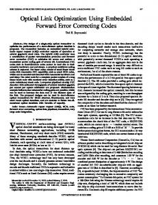
Figure 1.2: Obliquely angled corridors The principle of LP-based branch and bound is to exclude corridors which contain the current continuous optimum. Traditional branching on single variables leads to perpendicular corridors such as indicated by 1 in Figure 1.2, i.e., x1 ≤ 4 versus

≥5

(corridor 1).

An obliquely angled alternative [cf. MM83] would be corridor 2, i.e., 2x1 − x2 ≤ 6 versus

≥7

(corridor 2).

Corridors 1 and 2 have in common that they divide the solution set into subsets which have almost equally good continuous optima. This is due to the fact that the corridors are independent of the objective function. It seems to be advantageous to have corridors which are almost parallel to the objective function, such as x1 + x2 ≤ 6 versus ≥ 7 x1 + 2x2 ≤ 8 versus ≥ 9 x1 + 4x2 ≤ 13 versus ≥ 14

(corridor 3), (corridor 4), (corridor 5).

1

INTRODUCTION

5

These corridors were derived from the objective function. The coefficients were divided by constants and rounded. The right-hand-side bounds were selected such that the current continuous optimum was excluded. Many of the corridors constructed in this way have the property that feasible solutions lie only on one side of the corridor. This raises a corridor into the rank of a cutting plane (corridors 3, 4). The activation of corridor 4 would immediately lead to the discrete optimum. The effectiveness of a corridor can be measured by the decrease of the objective value of the continuous optimum and depends on several factors, in particular on • the angle between the corridor and the objective function, • the width of the corridor which depends directly on the coefficients of the variables (corr. 1: width 1, corr. 3: (1/2)0.5 = 0.707, corr. 2 and 4: (1/5)0.5 = 0.447, and corr. 5: (1/17)0.5 = 0.243), • the position of the excluded continuous optimum within the corridor. 1.3.1

Constructing basic corridors by d’Hondt ratios

To find strong corridors, we might need to construct many of them. Except for the simple method mentioned above, corridors can be constructed using d’Hondt ratios, a well-known technique used in political elections. The purpose of the corridors is to force those variables to integers which are basic in the continuous solution (slack variables are not considered). Therefore, basic corridors will be constructed by these variables only. Example 1.2. max

z z − 38x1 − 20x2 2x1 + 2x2 x1 2x1 − 2x2

− 41x3 + 2x3 − 3x3 + 5x3

− 35x4 + x4 + 5x4 + 3x4 x

= 0 ≤ 32 ≤ 2 ≤ 17 ∈ Z4+

An optimal LP solution is ( 161 , 102 , 41 , 0, 0, 0, 0). Thus, x1 –x3 are basic. 19 19 19 The d’Hondt ratios can be used to construct various corridors which are nearly parallel to the given source row. Let us take the objective as the source. Remember, we consider only x1 , x2 , x3 . The coefficients are divided by 1,2,3,4. . . and the results are written down, see Table 1.1. The numbers are ordered non-increasingly.

1

INTRODUCTION

6

In each step, 1 is added to the coefficient of the variable in the column with the next number, Table 1.2. We have considered two methods to construct integer corridors. The corridors obtained cannot exclude integer solutions (why?) 1.3.2

Bringing the branching constraints into the simplex tableau

As in the traditional branching, we need to select a strong corridor and integrate it into the simplex tableau. This procedure is the same here. We repeat it for completeness. Consider the first corridor (0,0,1). It means x3 ≤ 2, x3 ≥ 3. From the simplex tableau we can express x3 through the non-basic variables: 41 1 4 1 16 − x5 + x6 − x7 + x4 . 19 19 19 19 19 Now we take the first branch x3 ≤ 2 as x¯ = 2 − x3 ≥ 0 and express it through the non-basic variables. In this form it can be added to the simplex tableau. Moreover, we can compute the change of the objective function with one iteration of the dual simplex method. Doing this for all corridors and branches, we select the strongest corridor. x3 =

1.4

Modeling: Set Covering, Set Packing, Set Partitioning

Let M = {1 . . . m} be a finite set and and let {Mj } for j ∈ N = {1 . . . n} be a given collection of subsets of M . For example, the collections might consist of all subsets of size k for some k ≤ m. We say that F ⊆ N covers M if ∪j∈F Mj = M . We say that F ⊆ N is a packing with respect to M if Mj ∩Mk = ∅ for all j, k ∈ F ,

Table 1.1: D’Hondt ratios x1 x2 x3 si 38 20 41 q1i 38 20 41 q2i 19 10 20.5 q3i 12.67 6.67 13.67 q4i 9.5 5 10.25 ...

Table 1.2: Coefficients of the basic corridors no. x1 x2 x3 1 1 2 1 1 3 1 2 4 1 1 2 5 2 1 2 6 2 1 3 7 3 1 3 ...

LEC 2

2

1D CUTTING-STOCK PROBLEM (1D-CSP) Stock

Cutting plan

Cutting pattern

Length

Products

7

b1 b2 b3 Demand

Number of applications

Figure 2.1: 1D-CSP j 6= k. If F ⊆ N is both a covering and a packing, then F is said to be a partition of M . In the set-covering problem, cj is the cost of Mj and we seek a minimumcost cover; in the set-packing problem, however, cj is the weight or value of Mj and we seek a maximum-weight packing. These problems are readily formulated as 0-1 IPs. Let A be a m × n incidence matrix of the family {Mj } for j ∈ N ; that is, for i ∈ M , ( ( 1 if j ∈ F 1 if i ∈ Mj aij = xij = 0 if j 6∈ F 0 if i 6∈ Mj Then F is a cover (respectively packing, partition) iff x ∈ Bn satisfies Ax ≥ 1 (respectively Ax ≤ 1, Ax = 1). Many practical problems can be formulated as set-covering or similar problems.

2

1D Cutting-Stock Problem (1D-CSP)

Consider the one-dimensional cutting-stock problem (1D-CSP, Figure 2.1): given material pieces of length L and product lengths l1 ≥ l2 ≥ · · · ≥ lm , each demanded bi times, i = 1, . . . , m, find a packing of all products using the minimal number of stock pieces. In a real-life cutting process there are some further criteria, e.g., the number of different cutting patterns (setups), product due dates, minimal pattern run lengths, etc., see [JS04].

2

2.1

1D CUTTING-STOCK PROBLEM (1D-CSP)

8

The “Set-Covering” Model of 1D-CSP

This model arises naturally from the definition of a solution. A cutting pattern (Fig. 2.1) describes how many items of each type are cut from a stock length. Let column vectors aj = (a1j , . . . , amj ) ∈ Zm + , j = 1, . . . , n, represent all possible cutting patterns. To be a valid cutting pattern, aj must satisfy Pm (2.1) i=1 li aij ≤ L (knapsack condition). Let xj , j = 1, . . . , n, be the frequencies (i.e., the numbers of application) of the patterns in the solution. The model of Gilmore and Gomory (1961) is as follows: P (2.2a) z 1D−CSP = min nj=1 xj Pn i = 1, . . . , m (2.2b) s.t. j=1 aij xj ≥ bi , xj ∈ Z + ,

j = 1, . . . , n.

(2.2c)

This model has a non-polynomial number of variables. It can be written compactly:  z 1D−CSP = min cx : Ax ≥ b, x ∈ Zn+ . (2.3) Example 2.1. Consider the following 1D-CSP instance: (L = 4, m = 2, l = (2, 1), b = (2, 4)). The pattern matrix is   2 1 1 1 0 0 0 0 A= 0 2 1 0 4 3 2 1 The optimal solutions are (x1 = x5 = 1) and (x2 = 2).

2.2

Equivalence of 1D-CSP Instances

Two instances E1 = (L1 , m, l1 , b) and E2 = (L2 , m, l2 , b) are called equivalent (pattern-equivalent) if all feasible patterns for one instance are feasible for the other and vice versa [RST02]. Obviously one can obtain an equivalent instance multiplying all lengths by a positive constant or replacing L by L + ε or li by li − ε for a sufficiently small ε > 0. Hence the generality is not lost if L ∈ N and li ∈ N ∀i = 1 . . . m is demanded. Thus, further we assume L ∈ N, l ∈ Nm

and, moreover,

l1 > l2 > · · · > lm .

2

1D CUTTING-STOCK PROBLEM (1D-CSP)

9

Definition 2.1. A feasible pattern a is called maximal if L − la < lmin . Proposition 2.1. Two instances are equivalent iff they have equal sets of maximal patterns. However, it is difficult to formulate a practical criterion based on the maximal patterns of an unknown instance; instead, we use infeasible patterns of the original one. a > L, is called an infeasible pattern. ”ZV” Definition 2.2. A vector a ˇ ∈ Zm + , lˇ An infeasible pattern a ˇ is called minimal, if l˜ a ≤ L for all a ˜ a ˇ. und ”UZV” Proposition 2.2. Let A¯ = (¯ a1 | . . . |¯ an ) denote the maximal and Aˇ = (ˇ a1 | . . . |ˇ anˇ ) ¯ m, ¯l, b). Then the the minimal infeasible cutting patterns of the instance E¯ = (L, m instance E = (L, m, l, b) is equivalent to E¯ iff (l, L) ∈ Z+ × Z1+ is feasible for the inequalities l¯ aj ≤ L, j

lˇ a ≥ L + 1, li ≥ li+1 + 1, lm ≥ 1.

j = 1...n

(2.4a)

j = 1...n ˇ i = 1...m − 1

(2.4b) (2.4c) (2.4d)

Proof. “⇒” If E¯ and E are equivalent, (2.4a) follows from the definition of equiv- LEC 3 alence, (2.4b) holds because otherwise E has a feasible pattern which is infeasible ¯ and (2.4c) can be demanded to exclude symmetrical cases of E. in E, “⇐” With (2.4a), all feasible patterns of E¯ are feasible in E; with (2.4b), vice versa. Remark We can demand li ≥ li+1 in (2.4c) which increases the search space. However, for simplicity of the analysis, we consider strictly different lengths below. Now, to obtain an equivalent instance, it suffices to find out all maximal and min. infeasible patterns and solve (2.4). However, because of the condition l1 > · · · > lm , numerous constraints in (2.4) might automatically be fulfilled if other constraints are fulfilled as in the following     3 2 1 4 3 2 1 ¯ ˇ Example 2.2. Let A = . Then A = as in 1 2 3 1 2 3 4 the instance (15; 5, 4). From la1 ≤ L and l1 > l2 follows laj < L for j = 2 . . . 4. Analogously, from l(ˇ a5 ) ≥ L + 1 follows l(ˇ aj ) > L + 1 for j = 1 . . . 4. That means, only one inequality from each group (2.4a) and (2.4b) is needed, respectively.

2

1D CUTTING-STOCK PROBLEM (1D-CSP)

10

Exercise 2.1. For the instances (100;34,32,31) and (50;32,26,11), find the patterns which are sufficient for (2.4) to be true. Definition 2.3. A pattern a dominates cutting pattern a ¯ (abbreviation: a ≥d a ¯) m if la ≥ l¯ a for all l ∈ Z+ fulfilling l1 > · · · > lm . For a ∈ Zm let s0 (a) = 0, si (a) =

Pi

j=1

aj , i = 1 . . . m.

Lemma 2.3. For any given patterns a and a ¯ holds a ≥d a ¯ ⇔ si (a) ≥ si (¯ a),

i = 1 . . . m.

proof: exercise

Definition 2.4. Let the set of feasible patterns be fixed. Pattern a is called dominant if it is not dominated by any other feasible pattern. Note that a dominant pattern is maximal. Moreover, a dominant pattern can be characterized using the sizes (l, L) ∈ × Z1+ representing any certain instance with the corresponding feasible set. Let such l and L be given and l1 > · · · > lm . For any pattern a, define

Zm +

δ(a) = min{lm , li−1 − li : ai > 0, i = 2, . . . , m}. Lemma 2.4. Let A¯ represent a set of patterns and L ≥ l1 > · · · > lm represent ¯ A pattern a from A¯ is dominant iff some instance whose feasible set equals A. L − la < δ(a). Proof. “⇒” Assume L − la ≥ δ(a). Then there exists a feasible pattern a ˜ = a + em , if δ(a) = lm , or a ˜ = a + ei−1 − ei for some i = 2, . . . , m dominating a. “⇐” If a is not dominant then there exists a feasible pattern a ¯ 6= a with a ¯ ≥d a. The following three-step procedure can be applied iteratively: (i) If a ¯ ≥ a (component-wise), l¯ a − la ≥ lm ≥ δ(a), stop; (ii) Let j be the index determined by a ¯i = ai for i = 1 . . . j − 1 and a ¯j > aj . Define pattern e a with e aj = a ¯j −1, e aj+1 = a ¯j+1 +1, e ai = a ¯i for i 6∈ {j, j +1}. Then l¯ a − le a = lj − lj+1 and e aj+1 ≥ 1. (2.5) Furthermore, e a ≤d a ¯ since si (e a) = si (¯ a) for i 6= j and sj (e a) = sj (¯ a) − 1. Now, if e a = a then, because of (2.5), we have l¯ a − la ≥ δ(a) and hence, L − la ≥ δ(a). Otherwise set a ¯←e a and go to (i). Definition 2.5. An infeasible pattern a is called anti-dominant if it does not dominate any other infeasible pattern. Note that an anti-dominant pattern is minimal.

!l

i−1

li

−

2

1D CUTTING-STOCK PROBLEM (1D-CSP)

11

Anti-dominant patterns a ˇ can be identified similar to Lemma 2.4: the criterion is la − L ≤ δ(ˇ a) = min{li − li+1 : ai > 0, i = 1, . . . , m − 1, lm+1 ≡ 0}. Let Jd ⊂ {1 . . . n} denote the index set of dominant patterns in A¯ and Jnd ⊂ {1 . . . n ˇ} ˇ the index set of anti-dominant patterns in A. 1 Proposition 2.5. (l, L) ∈ Zm aj ≤ L for j ∈ Jd . + × Z+ fulfils (2.4a) iff l¯ j 1 m a ) ≥ L + 1 for j ∈ Jnd . Similarly, (l, L) ∈ Z+ × Z+ fulfils (2.4b) iff l(ˇ

Example 2.3. In order to illustrate the usage of dominance consider the instance EG = (10000; 5; (5000, 3750, 3250, 3001, 2000), (1, 1, 1, 1, 2)), ¯ EG has 41 feasible skip the cf. [RST02]. It has the IP-LP gap ∆(EG ) = 16 = 1.06. 15 patterns, among them are 20 maximal and 7 dominant. Moreover, it has 7 anti- rest dominant patterns. Hence, the class K(EG ) of equivalent instances can be described as a solution set of the system of inequalities: max{2l1 , l1 + 2l5 , 2l2 + l5 , l2 + 2l4 , l2 + 3l5 , 3l3 , 5l5 } ≤ L, min{l1 + l4 + l5 , l1 + 3l5 , 2l2 + l4 , l2 + l3 + l4 , 2l4 + 2l5 , l4 + 4l5 , 6l5 } ≥ L + 1, li ≥ li+1 + 1, i = 1 . . . 4, l5 ≥ 1, li ∈ Z+ , i = 1 . . . 5. One can look for a solution with the minimal L using the dual simplex method, e.g., with the optimization suite CPLEX: skip in lecture, only the ILOG CPLEX 9.100, licensed to "tu-dresden", options: e m b q CPLEX> display prob all result Minimize obj: L Subject To c1: - L + 2 l1 = 1 c15: l1 - l2 >= 1 c16: l2 - l3 >= 1 c17: - l4 + l3 >= 1 c18: - l5 + l4 >= 1 c19: l5 >= 1 Bounds All variables are >= 0.

2

1D CUTTING-STOCK PROBLEM (1D-CSP)

12

CPLEX> opt Tried aggregator 1 time. LP Presolve eliminated 1 rows and 0 columns. Reduced LP has 18 rows, 6 columns, and 48 nonzeros. Presolve time = 0.00 sec. Iteration log . . . Iteration: 1 Dual objective

=

5.000000

Dual simplex - Optimal: Objective = 6.0000000000e+01 Solution time = 0.00 sec. Iterations = 10 (0) CPLEX> disp sol var L-l3 Variable Name Solution Value L 60.000000 l1 30.000000 l5 12.000000 l2 22.000000 l4 19.000000 l3 20.000000

In this example, the LP solution is integer. Generally it might not be so. Then we need to apply integer programming methods. Give the result Note Similar transformations can be done in higher-dimensional problems, e.g., the pallet loading problem [Dow84, Sch08a]. Solving the equivalence problem for larger instances For real-size problems the number of maximal/(anti-)dominant patterns is very LEC 4 large. Then we can solve (2.4) by (dynamic) constraint generation. Let A1 be some initial set of maximal/infeasible patterns. It can be obtained by a simple heuristic. Or we simply start with the ordering constraints (2.4c). With these constraints, we solve the LP and obtain some values L, l1 . . . lm . To find if any other patterns violate (2.4a) or (2.4b), we can solve ¯ a ∈ Zm z¯ = max{la : ¯la ≤ L, + }, ¯ + 1, a ∈ Zm } z = min{la : ¯la ≥ L +

(2.6) (2.7)

and add patterns with z¯ > L + ε and z < L + 1 − ε. Note that (2.6) is a knapsack problem and (2.7) is a shortest path problem in a special graph. Both can be solved by dynamic programming, e.g., with the Gilmore-Gomory recursion [GG66, MT90].

3

EXACT APPROACHES FOR TSP

13 Not read

A very simple dynamic programming algorithm for (2.6) Function DP KP(L, l, d) Output: z¯, a ∈ Zm + v=k=0 for p = 0 to L − min{li } for i = 1 to m if vp + di > vp+li then vp+li = vp + di ; kp+li = i z¯ = vL restore a from k The complexity of the algorithm is O(Ln) (pseudo-polynomial). Lemma 2.6. With the strict sorting condition li ≥ li+1 + 1, i = 1 . . . m − 1 (2.4c), problems (2.6), (2.7) produce dominant/anti-dominant patterns, respectively. exercise

3

Exact Approaches for TSP

The TSP is one of the most widely studied combinatorial optimization problems [NW88]. Its statement is deceptively simple, and yet it remains one of the most challenging problems in Operations Research. It is a special case of some other problems (job sequencing, vehicle routing, etc.) Let G = (V, A) be a graph where V is a set of n vertices. A is a set of arcs or edges, and let C = (cij ) be a distance (or cost) matrix associated with A. The TSP is to find a minimal distance circuit passing through each vertex exactly once. Such a circuit is known as a tour or Hamiltonian circuit. C (and the problem) is symmetric (STSP) if cij = cji for all i, j ∈ V , and asymmetric otherwise (ATSP). Also, C is said to satisfy the triangle inequality iff cij + cjk ≥ cik for all i, j, k ∈ V (the metric TSP). This occurs, e.g., in Euclidian or geometric TSP where V corresponds to a set of points in R2 and cij is the straight-line distance between i and j.

3.1

Formulations of the Asymmetric TSP

We are going to consider some of the so-called double-index formulations [cf. GP02].

3

EXACT APPROACHES FOR TSP

14

Define the variables ( 1, xij = 0, The integer program P min i,j cij xij P s.t. x =1 Pi ij j xji = 1

if arc (i, j) is in the tour, otherwise. (3.1a) ∀j, ∀i,

(3.1b) (3.1c)

0 ≤ xij ≤ 1, xij integer, (3.1d) is a model of the assignment problem. The constraints of (3.1) are called the degree or assignment constraints. The constraint matrix of (3.1) is totally unimodular [STD-LEC] which means that there is always an integer optimal solution to the LP relaxation. Moreover, there are specialized algorithms with O(n3 ) running time. However, these solutions may contain several directed cycles, called subtours. One of the oldest branch&bound methods for ATSP used to break the subtours edge by edge, cf. [STD-LEC]. 3.1.1

The subtour formulation.

It was proposed by Dantzig, Fulkerson and Johnson in 1954 (DFJ formulation) and is used in to-day exact codes (see the TSP Home www.tsp.gatech.edu). A possible way to exclude subtours is to add to (3.1) the family of subtour (or subtour elimination) constraints (SECs) X xij ≤ |S| − 1 (S ( V, |S| > 1), (3.2) i,j∈S

to obtain the subtour formulation of the TSP consisting of (3.1) and (3.2). The relax disadvantage of its exponential size is mitigated by the fact that not all subtour inequalities must be put into the formulation from the start. They can be generated as needed by a separation algorithm: one can start with the formulation (3.1), then generate subtour inequalities that are violated by the current LP solution. 3.1.2

The MTZ formulation.

It was proposed by Miller, Tucker and Zemlin in 1960. To exclude subtours, one can use extra variables ui (i = 1, . . . , n), and the constraints u1 = 1, (3.3a) 2 ≤ ui ≤ n ∀i 6= 1, (3.3b) ui − uj + 1 ≤ (n − 1)(1 − xij ) ∀i 6= 1, ∀j 6= 1. (3.3c)

3

EXACT APPROACHES FOR TSP

15

We call (3.3c) an arc-constraint. The formulation consisting of (3.1) and (3.3) indeed excludes subtours, as (1) the arc-constraint for (i, j) forces uj ≥ ui + 1, when xij = 1; (2) if a feasible solution of (3.1), (3.3) contained more than one subtour, then at least one of these would not contain node 1, and along this subtour the ui values would have to increase to infinity. This argument, with the bounds on the ui variables, also implies that the only feasible value of ui is the position of node i in the tour. The advantages of the MTZ formulation are • its small size (we need only n extra variables and roughly n2 /2 extra constraints), • if it is preferable to visit, say, city i early in the tour, one can easily model this by adding a term αui with some α > 0 to the objective. 3.1.3

The strength of the two formulations.

One of the most important skills that a practitioner of integer programming must relax! acquire is that of designing a strong formulation for a particular problem. The main component of all commercial IP solvers is a branch-and-bound algorithm that uses the linear programming (LP) relaxation of an IP (i.e., the problem obtained from an IP by discarding the integrality constraints). Hence, a stronger formulation usually can be solved with fewer branch-and-bound nodes; if the tighter LPs are not “much” more time-consuming, this translates into a smaller overall solution time. Even if the problem cannot be solved to optimality within the available time, a strong formulation provides a good bound on the optimal value of the problem. Hence it can also serve as a counterpoint to an effective heuristic, by proving that a solution provided by the latter is close enough to being optimal. Solving a reasonably large (with at least, say, 50 cities) TSP instance to optimality is only possible using the subtour formulation; at least, we are not aware of any published computational studies that use the pure MTZ formulation. There is an analytical explanation of this fact: the LP relaxation of the MTZ formulation is much weaker. Since it contains the extra ui variables, for the comparison we need continue to eliminate them by taking appropriate linear combinations of the inequalities in here (3.1), (3.3). One way of doing this is by summing the arc-inequalities along a directed cycle. If the arc set of the cycle is denoted by C, then the result is X n−2 xij ≤ |C| (3.4) n−1 (i,j)∈C

On the other hand, if we denote the node set of the cycle by N (C), then the subtour formulation contains the obviously stronger inequality X xij ≤ |C| − 1. i,j∈N (C)

3

EXACT APPROACHES FOR TSP

16

The intuitive fact that adding the arc-inequalities along a cycle is the only “es- skipped sential” way to eliminate the ui variables can be made precise. Balas (2001) and in lec. Padberg and Sung (1991) showed that all nondominated inequalities in the projection of the MTZ formulation onto the space of the x variables are of the form (3.4). Thus, although the set of integer solutions in both models is the same, the set of LP solutions in the DFJ formulation is properly smaller.

3.2

The Subtour Formulation of the Symmetric TSP

When using the DFJ formulation for STSP, a solution of the LP relaxation typically contains many 2-node subtours. The symmetric problem is better handled by specialized algorithms that exploit its structure. Thus, variables xij are defined only for iP < j. For a set of edges E ⊆ {(i, j) : i < j}, define the sum of flows x(E) = (i,j)∈E xij . For a vertex set S, define δ(S) as the set of edges with one end in S and the other in S¯ = V \ S, the so-called S − S¯ cut. The subtour formulation is P (3.5a) zSTSP = min i 0.

4.2

TSP Heuristics with Good Empirical Performance

There are heuristics for TSP producing near-optimal solutions even for large instances. Most of them are based on local search. The classical local search structure is the k-exchange: remove k edges from the route and reconnect the tour in all possible ways. Example 4.3. Investigate the cases k = 2 and k = 3 graphically. The task is to organize the local search. One of the first successful strategies is the Lin-Kernighan heuristic. More sophisticated local search methods exist, e.g., chain ejection is applied in various combinatorial optimization problems.

5

Polyhedra and Valid Inequalities

In integer programming, we are typically given a set S ⊆ Zn+ of feasible points described implicitly, e.g., the set of integer solutions to a linear inequality system S = {x ∈ Zn+ : Ax ≤ b}, the set of binary vectors corresponding to tours in a graph, and so on. One of our objectives is to find a linear inequality description of S (see [STD-LEC]).

5.1

Definitions

Definition 5.1. A polyhedron P ⊆ Rn is the set of points that satisfy a finite LEC 7 number of linear inequalities; i.e., P = {x ∈ Rn : Ax ≤ b}, where (A, b) is an m×(n+1) matrix. A polyhedron is said to be rational if there exists an m0 ×(n+1) matrix (A0 , b0 ) with rational coefficients such that P = {x ∈ Rn : A0 x ≤ b0 }. Throughout the text we assume that if P is stated as {x ∈ Rn : Ax ≤ b}, then (A, b) has rational coefficients. Definition 5.2. A polyhedron P ⊆ Rn is called bounded if there exists an ω ∈ R1 such that P ⊆ {x ∈ Rn : −ω ≤ xj ≤ ω for j = 1, . . . , n}. A bounded polyhedron is called a polytope. Definition 5.3. A P set of points x1P , . . . , xk ∈ Rn is affinely independent if the k i unique solution of i=1 αi x = 0, ki=1 αi = 0 is αi = 0 for i = 1, . . . , k.

5

POLYHEDRA AND VALID INEQUALITIES

23

Linear independence implies affine independence, but the converse is not true. Proposition 5.1. The following statements are equivalent: a. x1 , . . . , xk ∈ Rn are affinely independent. b. x2 − x1 , . . . , xk − x1 are linearly independent. c. (x1 , −1), . . . , (xk , −1) ∈ Rn+1 are linearly independent. Note that the maximum number of affinely independent points in Rn is n + 1 (e.g., n linearly independent points and 0). Proposition 5.2. If {x ∈ Rn : Ax = b} = 6 ∅, the maximum number of affinely independent solutions of Ax = b is n + 1 − rank(A). Proposition 5.3. The following statements are equivalent: (i) {x ∈ Rn : Ax = b} = 6 ∅. (ii) rank(A) = rank(A, b). Definition 5.4. A polyhedron P is of dimension k, denoted dim(P ) = k, if the maximal number of affinely independent points in P is k + 1. Definition 5.5. A polyhedron P ⊆ Rn is full-dimensional if dim(P ) = n. Below we will show that if P is not full-dimensional, then at least one of the inequalities ai x ≤ bi is satisfied at equality by all points of P . Let M = {1, 2, . . . , m}, M = = {i ∈ M : ai x = bi for all x ∈ P } and ≤ M = {i ∈ M : ai x < bi for some x ∈ P } = M \ M = . Let (A= , b= ), (A≤ , b≤ ) be the corresponding rows of (A, b). We refer to the equality and inequality sets of representation (A, b) of P , that is, P = {x ∈ Rn : A≤ x ≤ b≤ , A= x = b= }. Note that if i ∈ M ≤ , then (ai , bi ) cannot be written as a linear combination of the rows of (A= , b= ). Now we relate dim(P ) to the rank of its equality matrix (A= , b= ). Below we always assume that P 6= ∅. Proposition 5.4. If P ⊆ Rn , then dim(P ) + rank(A= , b= ) = n. For proof, see [STD-LEC].

5

POLYHEDRA AND VALID INEQUALITIES

5.2

24

Describing Polyhedra by Facets

Given a polyhedron P = {x ∈ Rn : Ax ≤ b}, the question we address below is to find out which of the inequalities ai x ≤ bi are necessary in the description of P and which can be dropped. Definition 5.6. The inequality πx ≤ π0 [or (π, π0 )] is called a valid inequality for P if it is satisfied by all points in P . Note that (π, π0 ) is a valid inequality iff P lies in the half-space {x ∈ Rn : πx ≤ π0 } or equivalently iff max{πx : x ∈ P } ≤ π0 . Definition 5.7. If (π, π0 ) is a valid inequality for P , and F = {x ∈ P : πx = π0 }, F is called a face of P , and we say that (π, π0 ) represents F . A face F is said to be proper if F 6= ∅ and F 6= P . The face F represented by (π, π0 ) is nonempty iff max{πx : x ∈ P } = π0 . When F is nonempty, we say that (π, π0 ) supports P . We consider only supporting inequalities from now on. Definition 5.8. A face F of P is a facet of P if dim(F ) = dim(P ) − 1. Definition 5.9. We say that two valid inequalities (π, π0 ) and (λ, λ0 ) are equivalent, or identical inequalities with respect to P when (π, π0 ) = α(λ, λ0 ) + = u(A= , b= ) for some α > 0 and u ∈ R|M | . The definition of equivalent inequalities is motivated by the following Theorem 5.5. Let (A= , b= ) be the equality set of P ⊆ Rn and let F = {x ∈ P : πx = π0 } be a proper face of P . The following two statements are equivalent: i. F is a facet of P . ii. If λx = λ0 for all x ∈ F then =

(λ, λ0 ) = (απ + uA= , απ0 + ub= ) for some α ∈ R1 and some u ∈ R|M | . (5.1)

For proof, see [STD-LEC].

5

POLYHEDRA AND VALID INEQUALITIES

25

Example 5.1. Suppose P ⊆ R3 is given by Ax ≤ b with   1 1 1 1  −1 −1 −1 −1     1 0 1 1    0  0 0 (A|b) =  −1  0 −1 0 0     0 0 1 2  1 1 2 2 The three points (1 0 0), (0 1 0), (0 0 1) lie in P and are aff.ind. Hence dim(P ) ≥ 2. Because all points of P satisfy the equality x1 + x2 + x3 = 1, we have rank(A= , b= ) ≥ 1; hence, by Proposition 5.4, dim(P ) ≤ 2. P has at least two minimal descriptions: x1 + x2 + x3 = 1 −x1 ≤ 0 x1 + x3 ≤ 1

or

x1 + x2 + x3 = 1 −x1 ≤ 0 − x2 ≤ 0

Here the two last inequalities are equivalent with respect to P . In other words, a proper face is a facet exactly when, given any any equation representing F , all other such equations can be obtained from it by scaling and adding linear combinations of the equality constraints. Especially, if M = = ∅, that equation is unique.

5.3

Valid Inequalities for Integer Programs

We consider the discrete optimization problem max{cx : x ∈ S}, where S ⊆ Zn+ , and we formulate it as a linear integer program by specifying a rational polyhedron P = {x ∈ Rn+ : Ax ≤ b} such that S = Zn ∩ P . The topics to be studied concern the representation of an integer program by a linear program that has the same optimal solution. In [STD-LEC] we established the existence of such a representation: max{cx : x ∈ S} = max{cx : x ∈ conv(S)}. Definition 5.10. The valid inequalities (π, π0 ) and (γ, γ0 ) are said to be equivalent = if (π, π0 ) = λ(γ, γ0 ) + u(A= , b= ) for some λ > 0 and u ∈ R|M | . If they are not = equivalent and there exists µ > 0 and u ∈ R|M | such that γ ≥ µπ + uA= and γ0 ≤ µπ0 + ub= , then {x ∈ Rn+ : A= x = b= , γx ≤ γ0 } ⊆ {x ∈ Rn+ : A= x = b= , πx ≤ π0 }. In this case we say that γx ≤ γ0 dominates πx ≤ π0 . A maximal valid inequality is one that is not dominated by any other.

5

POLYHEDRA AND VALID INEQUALITIES

Example 5.2. S = {x ∈ Zn+ : Ax ≤ b}.   −1 2 1 , A= 5 −2 −2

26





4 b =  20  . −7

skip lec

We have             2 2 3 3 3 4 S= , , , , , = {x1 , . . . , x6 }. 2 3 1 2 3 0 conv(S) is a polytope defined by the 4 extreme points         2 2 3 4 , , , . 2 3 3 0 In this small example, it is easy to obtain a linear inequality representation of conv(S) from the four lines defined by the adjacent pairs of extreme points. The valid inequality 3x1 + 4x2 ≤ 24 is not maximal since it is dominated by the maximal valid inequality x1 + x2 ≤ 6. The valid inequality x1 ≤ 4 defines the zero-dimensional face {(4 0)}, but it is not maximal since it is dominated by the facet-defining inequality 3x1 + x2 ≤ 12. 5.3.1

Valid inequalities for the STSP polytope

Again, consider STSP defined on the complete undirected graph G = (V, E) with n nodes and m = n(n − 1)/2 edges. All validity proofs remain valid even for uncomplete graphs; however facet-defining properties not. We represent subsets of edges by their characteristic vectors x ∈ Bm (B = 0 0 0 {0, 1}) so that E 0 is represented by the vector xE , where xE e = 1 if e ∈ E and 0 xE e = 0 otherwise. Thus the set of feasible solutions S is the set of characteristic vectors whose edge sets induce tours. Let T = {x ∈ Bm : x ≤ x0 for some x0 ∈ S}. Note that T is the independence system [STD-LEC] whose maximal members define S. Because T ⊃ S, any valid inequality for T is also valid for S. Since 0 ∈ T and the m unit vectors are in T , dim(conv(T )) = m. Our reason for considering T is that conv(T ) is full-dimensional and thus easier to analyze than conv(S), which is not. Later in this section we show that dim(conv(S)) = m − n. T is also of practical interest since we can construct an objective function such that x0 is optimal over S iff x0 is optimal over T . Proposition 5.6. For any c ∈ Rm and ∞ > ω > max{|ce | : e ∈ E}, the following statements are equivalent.

LEC 8

in

5

POLYHEDRA AND VALID INEQUALITIES

27

1. x0 is an optimal solution to the STSP min{cx : x ∈ S}. 2. x0 is an optimal solution to max{¯ cx : x ∈ S}, where c¯e = ω − ce for all e ∈ E. 3. x0 is an optimal solution to max{¯ cx : x ∈ T }. Proof. 1 ⇔ 2. x0 is an optimal solution to the STSP min{cx : x ∈ S} iff x0 is P an optimal solution to max{−cx : x ∈ S}. But for any x ∈ S we have ω e∈E xe = nω. 2 ⇔ 3: because of c¯ > 0. We begin our study by first considering the lower- and upper-bound constraints xe ≥ 0 e ∈ E, xe ≤ 1 e ∈ E,

(5.2) (5.3)

which are obviously valid for S and T . Proposition 5.7. For all e ∈ E, (5.2) and (5.3) give facets of conv(T ). 0

Proof. Consider any e, e0 ∈ E. We have x{e,e } ∈ T . The m vectors x{e} and 0 x{e,e } for all e0 6= e are linearly independent and satisfy xe = 1. Hence, all of the inequalities (5.3) are facets. 0 (5.2): the m points x{e } for e0 6= e and 0 are affinely independent. The relative complexity of conv(S) is already seen by observing that for n = 3, conv(S) contains the single point x = (111), so, for example, (5.2) is not even a supporting hyperplane for any e ∈ E. It can be shown, however, that (5.2) yields facets of conv(S) when n ≥ 5, and all (5.3) yield facets for n ≥ 4. Now consider the degree constraints x(δ(i)) = 2 x(δ(i)) ≤ 2

i ∈ V, i ∈ V,

(5.4) (5.5)

for S and T , respectively. Proposition 5.8. For all i ∈ V , (5.5) gives a facet of conv(T ). Proof. Suppose that δ(i) = {e1 . . . , en−1 } and that {e1 , e2 , em } forms a cycle. Consider the m vectors: x{e1 ,ej } for j = 2, . . . , n − 1; x{e2 ,e3 } , x{e1 ,e2 ,ej } for j = n, . . . , m−1; and x{e1 ,e3 ,em } . Each of these vectors is in T and satisfies (5.5) at equality, and it is easy to check that they are linearly independent. (exercise) Proposition 5.9. dim(conv(S)) = m − n = n(n − 1)/2 − n.

5

POLYHEDRA AND VALID INEQUALITIES

28

Proof. Let Q = {x ∈ Bm : x satisfies (5.4)}. The equation system (5.4) defines a constraint matrix of rank n. By Proposition 5.4, we have dim(conv(Q)) = m − n. Since conv(S) ⊆ conv(Q), it follows that dim(conv(S)) ≤ m − n. To prove that dim(conv(S)) = dim(conv(Q)) = m − n, it suffices to show that if the hyperplane πx = π0 , π 6= 0, contains the incidence vector of every tour, then πx = π0 is a linear combination of the constraints (5.4). The edge set of the graph G is E = {(i, j) : i = 1, . . . , n−1, j = i+1, . . . , n}. The variable xe for e = (i, j) is written as xij . Let j ∈ {4, . . . , n} and Pj3 be a path from j to 3 through all of the points {4, . . . , n}. Now consider the pairs of tours Tj1 = Pj3 ∪ {(1, j), (1, 2), (2, 3)} and Tj2 = Pj3 ∪ {(2, j), (1, 2), (1, 3)}, shown in Figure 5.1. Since Tj1 and Tj2 lie on the hyperplane πx = π0 , it follows that π1j + π23 = π2j + π13 or π2j − π1j = π23 − π13 for j = 3, . . . , n. Let λ1 = π2j − π1j for j = 3, . . . , n. By an identical argument, we obtain the following for i = 1, . . . , n: λi = πi+1,j − πij for j > i + 1 and λi = πj,i+1 − πji for j < i.

j

1

j

1

3

2

3

2

Figure 5.1:

Thus for any coefficient πij , we have πij = (πij − πi−1,j ) + πi−1,j = (πij − πi−1,j ) + · · · + (π2j − π1j ) + π1j P = i−1 t=1 λt + π1j Pi−1 = t=1 λt + (π1j − π1,j−1 ) + π1,j−1 P = i−1 t=1 λt + (π1j − π1,j−1 ) + · · · + (π13 − π12 ) + π12 Pi−1 P = t=1 λt + j−1 t=2 λt + π12 = ui + uj − u2 + π12 , Pi−1 where ui = t=1 λt for i > 1 and u1 = 0. Let α = π12 − u2 . Hence P Pn−1 Pn Pn−1 Pn e∈E πe xe = i=1 j=i+1 πij xij = i=1 j=i+1 (ui + uj + α)xij

 P P Pn  = i=1 ui + α2 x + x ji ij ji
P α = v∈V uv + 2 x(δ(v)), which establishes P that the constraint is a linear combination of degree constraints with π0 = 2 v∈V uv + nα.

5

POLYHEDRA AND VALID INEQUALITIES

29 0

In a cycle, each vertex is of degree 2. Hence if xE ∈ Bm satisfies (5.4) for all v ∈ V , then the subgraph G0 = (V, E 0 ) is either a tour or a set of disjoint subtours. Consider again the subtour elimination constraint x(E(W )) ≤ |W | − 1

for all W ⊂ V, 2 ≤ |W | ≤ n − 1.

(5.6)

We include the case |W | = 2 although it is just the upper bound (5.3). In addition, if the degree constraints are satisfied, (5.6) are superfluous for all W with |W | > n/2. Proposition 5.10. The SECs (5.6) give facets of conv(S) for n ≥ 4 for all W ⊂ V with 2 ≤ |W | ≤ n/2. For proof, see [NW88]. 5.3.2

Integer rounding: special cases of Chv´atal-Gomory cuts 1

LP

e7

5

Rm +

: x satisfies degree, Let P = {x ∈ e5 e2 upper bound and SECs}. For n ≤ 5, it 3 6 e8 e1 e4 can be shown that conv(S) = P LP . A e3 e6 subgraph on six nodes is shown in Fig1 0 0 ure 5.2. The vector x with xei = 2 for e9 2 4 i = 1, . . . , 6, x0ei = 1 for i = 7, 8, 9, and x0ei = 0 otherwise is a feasible point in Figure 5.2: A subgraph on six nodes P LP . Exercise 5.1. Prove that x0 is an extreme point of P LP by showing that it is the unique optimal solution to min{cx : x ∈ P LP }, where cei = 1 for i = 1, . . . , 6, cei = 0 for i = 7, 8, 9, and cei is suitably large otherwise. To define a polytope that contains conv(S) but not x0 , we use the following LEC 9 argument. Summing up x(δ(i)) = 2 for i = 1, 2, 3, xei ≤ 1 for i = 7, 8, 9, and −xe ≤ 0 for all other edges with one end in {1, 2, 3} yields 2(xe1 + xe2 + xe3 + xe7 + xe8 + xe9 ) ≤ 9. For integer x, the left side is even. Thus, the right-hand side can be reduced to 8. P This inequality is a special case of the Chv´atal-Gomory cut j (buaj c)xj ≤ bubc [STD-LEC], also called integer rounding. We can use integer rounding to generalize the example of Figure 5.2. Let H be any subset of nodes with 3 ≤ |H| ≤ |V | − 1 and let F ⊂ E be an odd set of disjoint edges, each of which has one end in H.

5

POLYHEDRA AND VALID INEQUALITIES

30

H

F

P Summing up the degree constraints for all nodes in H: v∈H x(δ(v)) = 2x(E(H)) + x(δ(H)) = 2|H|, the nonnegativity constraints −x(δ(H) \ F ) ≤ 0, and the upper bounds x(F ) ≤ |F | and noting that x(δ(H)\F ) = x(δ(H))−x(F ) gives 2x(E(H)) + x(δ(H)) − x(δ(H) \ F ) + x(F ) ≤ 2|H| + |F | ⇐⇒ 2x(E(H)) + 2x(F ) ≤ 2|H| + |F |; the left-hand side is even, and so should be the right-hand side. However, we demanded |F | to be odd! Thus, 2x(E(H)) + 2x(F ) ≤ 2|H| + |F | − 1

(5.7)

holds. We can subtract 2x(E(H)) + x(δ(H)) = 2|H| to obtain equivalent forms or

2x(F ) ≤ x(δ(H)) + |F | − 1 x(F ) ≤ x(δ(H) \ F ) + |F | − 1

(5.8) (5.9)

which reads as xe7 + xe8 + xe9 ≤ x(δ(H) \ F ) + 2 in the example of Figure 5.2. Now we have that conv(S) ⊆ P1LP = {x ∈ P LP : x satisfies (5.7)}. In fact it can be shown that P1LP = conv(S) on all graphs with six or fewer nodes. But, for n ≥ 7, more general inequalities are needed, e.g., by using SECs in the combination. 5.3.3

Valid inequalities from combinatorial implications

In quite many cases, effective cuts can be obtained by logical arguments using the problem structure. Consider the node-packing problem: a set of nodes in a graph G = (V, E) is a packing if no two nodes are joined by an edge (interpret as set packing: exercise). Thus, the set of node packings is given by S = {x ∈ Bn : xi + xj ≤ 1 ∀(i, j) ∈ E}

(5.10)

5

POLYHEDRA AND VALID INEQUALITIES

31

2 6

3

Figure 5.3: 1 4

5

where n = |V |. The vector x ∈ S is the characteristic vector of a packing; i.e., xi = 1 if node i is in the packing and xi = 0 otherwise. Since S contains the zero vector and the n unit vectors, dim(conv(S)) = n. A set C ⊆ V is called a clique if each pair of nodes in C is joined by an edge. Thus a node packing can contain no more than one node from each clique. For the graph of Figure 5.3, the maximal cliques yield the inequalities     x1   1 1 1 1 x  1   2  1 1 1   x    1 1   3  ≤ 1 (5.11) 1 x4    1 1 1  1 x  5 1 1 1 1 x6 corresponding to the cliques 123, 134, 145, 156, and 126. Proposition 5.11. When C is a maximal clique, the clique constraint X xj ≤ 1

(5.12)

j∈C

defines a facet of conv(S). Proof. Using definition of a facet directly. Suppose that C = {1, . . . , k}. Since C is maximal, for each j 6∈ C there is a node l(j) such that l(j) ≤ k and {j, l(j)} is a node packing. The characteristic vectors of the packings {1}, . . . , {k}, {k + 1, l(k + 1)}, . . . , {n, l(n)} are easily shown to be linearly independent. The rows of the matrix given below are six linearly independent vectors which establish that x1 + x2 + x3 ≤ 1 is facet for the graph of Figure 5.3.   1  1    1    1  1    1 1  1 1

5

POLYHEDRA AND VALID INEQUALITIES

32

Although there is an important class of node-packing problems for which the maximal clique constraints and nonnegativity give all the facets of conv(S), this is not true in our example. In particular, x1 = 12 (0 1 1 1 1 1) is an extreme point of the polytope given by (5.11) and x ≥ 0. This can be seen by solving the linear program max 1x subject to (5.11) and x ≥ 0. The unique optimum is x1 . To cut off x1 , we consider another family of valid inequalities. Suppose there is an H ⊆ V that induces a chordless cycle, that is, the nodes of H can be ordered as (i1 , i2 , . . . , ip ) such that (ir , is ) ∈ E iff s = r + 1 or s = 1 and r = p. If p is odd and at least 5, then H is called an odd hole. If H is an odd hole, then X |H| − 1 xj ≤ (5.13) 2 j∈H is satisfied by all node packings. Moreover, the clique constraints xi + xj ≤ 1 for i, j ∈ H do not imply (5.13). In our example, H = {23456} is an odd hole an we obtain x2 + x3 + x4 + x5 + x6 ≤ 2

(5.14)

which cuts off x1 . Since (5.14) is satisfied at equality by the five linearly independent characteristic vectors corresponding to the packings 24, 25, 35, 36, and 46, inequality (5.14) gives a facet of the convex hull of node packings for the subgraph with node set H. But it does not give a facet of conv(S) for the graph G, since there are no other packings that satisfy (5.14) at equality. If we added (5.14) to the clique constraints, we would obtain the new extreme point 15 (1 2 2 2 2 2). 5.3.4

Lifting

Since (5.14) is a four-dimensional face of conv(S) but not a facet, it can perhaps be strengthened by tilting it to produce a facet. In other words, is there a valid inequality of the form αx1 + (x2 + x3 + x4 + x5 + x6 ) ≤ 2

(5.15)

with α > 0? And if so, what is the largest value of α that preserves validity? To LEC 10 answer these questions, we must consider x1 = 0 and x1 = 1. When x1 = 0, (5.15) is valid for any α > 0. When x1 = 1, we have α ≤ 2 − (x2 + x3 + x4 + x5 + x6 ). But x1 = 1 implies x2 = · · · = x6 = 0, so α ≤ 2. Thus 2x1 + (x2 + x3 + x4 + x5 + x6 ) ≤ 2

(5.16)

5

POLYHEDRA AND VALID INEQUALITIES

33

is a valid inequality. Moreover, it gives a facet of conv(S) since it is satisfied at equality by the characteristic vector of {1} and the five characteristic vectors for (5.14). We have just illustrated a general principle called lifting whereby a valid inequality for S ∩ {x ∈ Bn : x1 = 0} is extended to a valid inequality for S. Proposition 5.12. Suppose S ⊆ Bn , S δ = S ∩ {x ∈ Bn : x1 = δ} for δ ∈ {0, 1}, and Pn (5.17) j=2 πj xj ≤ π0 is valid for S 0 . If S 1 = ∅, then x1 ≤ 0 is valid for S. If S 1 = 6 ∅, then Pn α1 x1 + j=2 πj xj ≤ π0 (5.18) P is valid for S for any α1 ≤ π0 − ζ 0 , where ζ 0 = max{ nj=2 πj xj : x ∈ S 1 }. Moreover, if α1 = π0 − ζ 0 and (5.17) gives a face of dimension k of conv(S 0 ), then (5.18) gives a face of dimension k + 1 of conv(S). Proof. If x¯ ∈ S 0 , then P P α1 x¯1 + nj=2 πj x¯j = nj=2 πj x¯j ≤ π0 since (5.17) is valid for S 0 . If x¯ ∈ S 1 , then P P α1 x¯1 + nj=2 πj x¯j = α1 + nj=2 πj x¯j ≤ α1 + ζ 0 ≤ π0 by definition of the quantities α1 and ζ 0 . Since (5.17) gives a k-dimensional face of conv(S 0 ), there exist xi ∈ S for i = 1, . . . , k + 1 that are affinely independent and satisfy (5.17) at equality. Since xi1 = P 0, it follows that xi satisfies (5.18) at equality for i = 1, . . . , k + 1. Let 0 ζ = nj=2 πj x∗j , where x∗ ∈ S 1 . With α1 = π0 − ζ 0 , x∗ satisfies (5.18) at equality. Finally, since x∗1 = 1, it follows that x∗ cannot be written as an affine transformation of {x1 , . . . , xk+1 }, so the k + 2 vectors {x∗ , x1 , . . . , xk+1 } are affinely independent. The lifting principle is also applicable to extending a valid inequality from S 1 to S. We can use Proposition 5.12 with the complement variable x1 = 1 − x1 (exercise) to show: Proposition 5.13. Suppose (5.17) is valid for S 1 . If S 0 = ∅, then x1 ≥ 1 is valid for S. If S 0 6= ∅, then P γ1 x1 + nj=2 πj xj ≤ π0 + γ1 (5.19) Pn 1 1 is valid for S for any γ1 ≥ ζ − π0 , where ζ = max{ j=2 πj xj : x ∈ S 0 }. Moreover, if γ1 = ζ 1 − π0 and (5.17) gives a face of dimension k of conv(S 1 ), then (5.19) gives a face of dimension k + 1 of conv(S).

5

POLYHEDRA AND VALID INEQUALITIES

34

When α1 = π0 − ζ 0 in Proposition 5.12 or when γ1 = ζ 1 − π0 in Proposition 5.13, we say that the lifting is maximum. Propositions 5.12 and 5.13 are meant to be used sequentially and the coefficients {αj } or {γj } depend on the order in which the variables are lifted. π2 6 (0, π20 )

π0 Q

Figure 5.4:

Q

Q

QQ

B

π1 B B

B B

π2 -

(0, 0) (π12 , 0)

π1

Geometric interpretation of lifting. It is insightful to examine the lifting 1 n n process Pn in the polar space Π =0 {π ∈ R : πx ≤ 1 for all x ∈ S ⊆ B }. If j=2 πj xj ≤ 1 is valid for S , maximum lifting can be described by the 1D optimization problem in Π1 -space: max{α : (0, π2 , . . . , πn ) + α(1, 0, . . . , 0) ∈ Π1 }. The geometry is illustrated in Figure 5.4 for the case n = 2. We suppose that Π1 has the three extreme points {π 0 , π 1 , π 2 }. Since π20 > max{π21 , π22 }, we have that π20 x2 ≤ 1 gives a facet of conv(S 0 ), where S 0 = S ∩ {x : x1 = 0}. Maximum lifting is equivalent to moving from (0, π20 ) in the direction (1 0) to obtain the extreme point π 0 of Π1 or, equivalently, the facet of conv(S) defined by π10 x1 + π20 x2 ≤ 1 (Proposition 5.12). Similarly, by a maximum lifting from π12 x1 ≤ 1, we obtain the facet defined by π 2 . Remark. The extreme points of Π1 correspond to facets of conv(S) (without proof). We see that sequential lifting cannot obtain the facet corresponding to π 1 . To interpret sequential lifting geometrically, suppose we begin with the trivial inequality 0 ≤ 1. Maximum lifting in the order (1, 2) yields the facet corresponding to the extreme point π 2 , and maximum lifting in the order (2, 1) yields π 0 Neither order gives π 1 . In principle, lifting is not restricted to choosing one coefficient at a time. If we observe that maximum sequential lifting is equivalent to finding an extreme

5

POLYHEDRA AND VALID INEQUALITIES

35

point in a one-dimensional polyhedron, it is not surprising that in the simultaneous lifting of k coefficients, the strongest inequalities are obtained as extreme points of a k-dimensional polyhedron. Hence if we start from the inequality 0 ≤ 1 and allow the simultaneous lifting of (π1 , π2 ), we can indeed obtain π 0 , π 1 , and π 2 . Maximum lifting is one of the methods to show the facet-defining property. 5.3.5

Valid inequalities for the 0-1 knapsack polytope: covers

We consider the constraint set of a 0-1 knapsack problem P S = {x ∈ Bn : j∈N aj xj ≤ b},

(5.20)

where N = {1, . . . , n}, aj ∈ Z1+ for j ∈ N , and b ∈ Z1+ . We can also consider the description of S as part of a constraint set of an IP problem so that the valid inequalities for S are valid for the whole problem. S is an independence system. Since aj > b implies xj = 0 for all x ∈ S, we assume aj ≤ b for all j ∈ N . Thus dim(conv(S)) = n. It is convenient to order the coefficients monotonically so that a1 ≥ a2 ≥ · · · ≥ an . We represent elements of Bn by characteristic vectors so that for R ⊆ N the vector xR has components C xR j = 1 iff j ∈ R. If x ∈ S, we say that C is an independent set; otherwise C is a dependent set or a cover. Exercise 5.2. Prove that the n constraints x ≥ 0 give facets of conv(S). In addition, xj ≤ 1 gives a facet if {j, k} is an independent set for all k ∈ N \{j}. Proposition 5.14. If C is a dependent set, then P j∈C xj ≤ |C| − 1

LEC 11 (5.21)

(the so-called cover inequality) is a valid inequality for S. A dependent set is minimal if all of its subsets are independent. Note that if a P dependent set is not minimal, then (5.21) is the sum of j∈C 0 xj ≤ |C 0 | − 1 and xj ≤ 1 for j ∈ C \ C 0 , where C 0 is a minimal dependent set. Example 5.3. S = {x ∈ B5 : 79x1 + 53x2 + 53x3 + 45x4 + 45x5 ≤ 178}. The minimal dependent sets and the corresponding valid inequalities are: C1 C2 C3 C4

= {1, 2, 3} = {1, 2, 4, 5} = {1, 3, 4, 5} = {2, 3, 4, 5}

x1 + x2 + x3 x1 + x2 + x4 + x5 x1 + x 3 + x4 + x5 x2 + x 3 + x4 + x5

≤ ≤ ≤ ≤

2 3 3 3.

5

POLYHEDRA AND VALID INEQUALITIES

36

While the constraints (5.21) are quite simple, they are nontrivial with respect to the polytope P ⊇ S obtained by replacing x ∈ Bn by P x ∈ Rn+ and xj ≤ 1 for all j ∈ N , that is, the LP relaxation with P = {x ∈ Rn+ : j∈N aj xj ≤ b, xj ≤ 1 for j ∈ N }. Exercise 5.3. Show that every nonintegral extreme point xˆ of P is of the form xˆj = 1 for j ∈ C \ {k} xˆj = 0 for j ∈ N \ C P xˆk = (b − j∈C\{k} aj )/ak > 0, where C is a cover, k ∈ C, and C \ {k} is independent. Hint: use either the definition of extreme point or construct a linear objective function so that xˆ is the unique solution to the relaxation. However, xˆ does not satisfy (5.21). Proposition 5.15. If C is a minimal cover then the inequality (5.21) defines a facet of conv(SC ) where SC = S ∩ {x : xj = 0, j ∈ N \ C}. Proposition 5.16. P If C is a minimal cover for S and (C1 , C2 ) is any partition of C with C1 6= ∅, then j∈C1 xj ≤ |C1 | − 1 gives a facet of conv(S(C1 , C2 )), where S(C1 , C2 ) = S ∩ {x ∈ Bn : xj = 0 for j ∈ N \ C, xj = 1 for j ∈ C2 }. Proof. For any C2 , ∅ ⊆ C2 ⊂ C, it follows that C1 = C \ C2 is a minimal dependent set for S(C1 , C2 ), since P P S(C1 , C2 ) = {x ∈ B|C1 | : j∈C1 aj xj ≤ b − j∈C2 aj }, P P P P j∈C1 aj > b − j∈C2 aj , and j∈C1 \{k} aj ≤ b − j∈C2 aj for all k ∈ C1 . Now apply the definition of facet. We can use Proposition 5.16 and lifting to generate facets of conv(S). Proposition 5.17. If C is a minimal cover for S and (C1 , C2 ) is any partition of C with C1 6= ∅, then conv(S) has a facet represented by P P P P j∈N \C αj xj + j∈C2 γj xj + j∈C1 xj ≤ |C1 | − 1 + j∈C2 γj , where αj ≥ 0 for all j ∈ N \ C and γj ≥ 0 for all j ∈ C2 .

5

POLYHEDRA AND VALID INEQUALITIES

37

P Proof. We start with the inequality j∈C1 xj ≤ |C1 | − 1, which gives a facet of conv(S(C1 , C2 )), and do lifting by applying Proposition 5.12 for each j ∈ N \ C and Proposition 5.13 for each j ∈ C2 . The nonnegativity of the coefficients is implied by their definitions in the Propositions. As we mentioned, the order of the variables in the lifting affects the coefficients. We should begin with P a j ∈ N \ C, because beginning with a k ∈ C2 is equivalent to starting with j∈C1 ∪{k} xj ≤ |C1 |. In Example 5.3, lifting x1 for C4 gives the facet x1 + x2 + x3 + x4 + x5 ≤ 3 which dominates C2 and C3 . Lifting x4 and x5 for C1 shows that x1 + x2 + x3 ≤ 2 is already a facet. Example 5.4. S = {x ∈ B5 : 3x1 + x2 + x3 + x4 + x5 ≤ 4}. a. C = {1, 4, 5} is a minimal cover. Lifting x2 and x3 gives the facet x1 + x4 + x5 ≤ 2 of conv(S). b. C = {1, 4, 5}, C1 = {4, 5}, C2 = {1}. By Proposition 5.16, x4 + x5 ≤ 1 gives a facet of conv{(x4 , x5 ) ∈ B2 : x4 +x5 ≤ 4−3 = 1} = conv{S∩{x ∈ B5 : x1 = 1, x2 = x3 = 0}}. First we lift x3 by applying Proposition 5.12: α3 = 1 − max{x4 + x5 : (x4 , x5 ) ∈ B2 , x4 + x5 ≤ 4 − 3x1 − x3 , x1 = x3 = 1}. Hence α3 = 1 and x3 + x4 + x5 ≤ 1 gives a facet of conv{x ∈ B3 : x3 + x4 + x5 ≤ 1}. Now we lift x1 by applying Proposition 5.13. Hence γ1 = max{x3 + x4 + x5 : x ∈ B3 , x3 + x4 + x5 ≤ 4} − 1 = 2. Thus 2x1 +x3 +x4 +x5 ≤ 3 gives a facet of conv{x ∈ B4 : 3x1 +x3 +x4 +x5 ≤ 4}. Finally, we lift x2 . α2 = 3 − max{2x1 + x3 + x4 + x5 : x ∈ B4 , 3x1 + x3 + x4 + x5 ≤ 3}. Thus α2 = 0 and 2x1 + x3 + x4 + x5 ≤ 3 gives a facet of conv(S). By symmetry, lifting in the order (x2 , x1 , x3 ) yields the same facet. The orders (x2 , x3 , x1 ) and (x3 , x2 , x1 ) show that the original inequality 3x1 + x2 + x3 + x4 + x5 ≤ 4 also gives a facet of conv(S). We have not considered lifting x1 first because, as explained before the example, this yields x1 + x4 + x5 ≤ 2, which we already know gives a facet. To apply Proposition 5.17, we must solve |N \ C1 | 0-1 knapsack problems. However, unlike the general 0-1 KP, these can be solved in polynomial time by dynamic programming, similar to the algorithm on page 13 because the constraint coefficients are polynomial in n.

5

POLYHEDRA AND VALID INEQUALITIES

38

Remark. In general, we cannot obtain all facets by sequential lifting (see Geometric interpretation of lifting). Proposition 5.17 applies to any independent system. We now begin to use some particular properties of the knapsack problem. In fact, we are going to simplify lifting in certain cases. Definition 5.11. The extension E(C) of a minimal cover C is the set C ∪ {k ∈ N \ C : ak ≥ aj for all j ∈ C}. In Example 5.3, E(Ci ) = Ci for i = 1, 2, 3 and E(C4 ) = C4 ∪ {1}. Proposition 5.18. If C is a minimal cover, then P j∈E(C) xj ≤ |C| − 1

(5.22)

is a valid inequality for S. P Proof. Suppose xR ∈ S and j∈E(C) xR ≥ |C|. Now j ≥ |C| so that |R ∩ E(C)| P P P a ≥ j∈R∩E(C) aj and by definition of E(C) we obtain j∈R∩E(C) aj ≥ Pj∈R j R j∈C aj > b, which contradicts x ∈ S. P In Example 5.3, 5j=1 xj ≤ 3 is a valid inequality obtained from Proposition 5.18 with E(C4 ). It dominates the inequalities (5.21) generated by C2 , C3 , and C4 . Proposition 5.19. Let C = {j1 , . . . , jr } be a minimal cover with j1 < j2 < · · · < jr . If any of the following conditions hold, then (5.22) gives a facet of conv(S). a. C = N . b. E(C) = N and (i) (C \ {j1 , j2 }) ∪ {1} is independent. c. C = E(C) and (ii) (C \ {j1 }) ∪ {p} is independent, where p = min{j : j ∈ N \ E(C)}. d. C ⊂ E(C) ⊂ N and (i) and (ii). Proof. Method 1. Use maximal lifting and the fact that the items are sorted. Method 2. Use the definition of facet and the following n linearly independent points which satisfy (5.22) at equality: 1. Ii = C \ {ji } for ji ∈ C. There are |C| of these. 2. Ik0 = (C \ {j1 , j2 }) ∪ {k} for k ∈ E(C) \ C. |Ik0 ∩ E(C)| = |C| − 1 and Ik0 LEC 12 is independent by (i) and ak ≤ a1 . There are |E(C) \ C| of these. 3. I˜j = (C \ {j1 }) ∪ {j} for j ∈ N \ E(C). |I˜j ∩ E(C)| = |C| − 1 and I˜j is independent by (ii) and aj ≤ ap .

5

POLYHEDRA AND VALID INEQUALITIES

39

The proof that the corresponding characteristic vectors are linearly independent is left as an exercise. In Example 5.3, Proposition 5.19 establishes that (5.22) with C = C1 gives a facet of conv(S) since C1 = E(C) and (C1 \ {j1 }) ∪ {p} = {2, 3, 4} is independent. Also, since E(C4 ) = N and (C4 \ {2, 3}) ∪ {1} = {1, 4, 5} is independent, (5.22) with C = C4 gives a facet of conv(S). In Example 5.4.a, C = {1, 4, 5} is a minimal cover and E(C) = {1, 4, 5}. By Proposition 5.19, x1 + x4 + x5 ≤ 2 gives a facet of conv(S). Exercise 5.4. For S = {x ∈ B6 : 5x1 + 5x2 + 5x3 + 5x4 + 3x5 + 8x6 ≤ 17} and C = {1, 2, 3, 4}, lift x5 and x6 in the two possible sequences and show that the resulting inequalities are facets of conv(S). 5.3.6

Lifted cover inequalities in 0-1 problems: branch-and-cut

The general 0-1 IP max{cx : Ax ≤ b, x ∈ Bn },

(BIP)

where A is an m × n integral matrix and b ∈ Zm , typically is solved by a general LP-based branch&bound. However, BIP possesses a few properties that can be used to refine a general algorithm and make it more efficient. Linear programming relaxations can yield more information for BIPs than for general IPs because of the following proposition. Proposition 5.20. Every feasible solution to (BIP) is an extreme point of P = {x ∈ Rn+ : Ax ≤ b, x ≤ 1}. Proof. If x is not extreme, then x = 21 x1 + 12 x2 , x1 , x2 ∈ P with x1 6= x2 , which implies 0 < xj < 1 for some j ∈ N ; that is, x 6∈ Bn . This result motivates a heuristic that systematically searches the integral extreme points of P in the neighborhood of an optimal solution to the LP relaxation. Another useful fact is that by complementing variables, the individual constraints of BIP can be written as the constraint sets of 0-1 knapsack problems. Specifically, the ith constraint can be restated as X X |aij |˜ x j ≤ bi − aij , x˜ ∈ Bn , (5.23) j∈N

j∈N :aij 0 and x˜j = 1 − xj if aij < 0. Thus, we can apply strong cuts for the 0-1 knapsack polytope.

5

POLYHEDRA AND VALID INEQUALITIES

40

In a node of a b&b tree, we solve the LP relaxation. Suppose its solution x∗ is non-integral. In such a case we can always branch. But, in order to reduce the number of explored nodes, we can try to tighten the formulation by cover cuts. The resulting algorithm then is of the type branch-and-cut. P P Formally, we want to find a C ⊂ N with j∈C aj > b and j∈C x∗j > |C|−1. IntroducingP a vector z ∈ Bn to represent the unknown set C, we attempt to choose P P ∗ z such that j∈N aj zj > b and j∈N xj zj > j∈N zj −1. The second inequality P is equivalent to j∈N (1 − x∗j )zj < 1. We obtain the separation problem for cover inequalities: nX o X θ = min (1 − x∗j )zj : (5.24) aj zj > b, z ∈ Bn . j∈N

j∈N

P Note that, since the constraint coefficients are integral, j∈N aj zj > b is equivaP lent to j∈N aj zj ≥ b + 1. To obtain stronger cuts, it is very effective to apply lifting leading to the facetdefining cuts P P P P (5.25) j∈C2 γj xj + j∈C1 xj ≤ |C1 | − 1 + j∈C2 γj , j∈N \C αj xj + with C1 ∩ C2 = ∅ and C1 ∪ C2 = C (see above). The coefficients {αj } and {γj } are obtained by maximal sequential lifting. Unfortunately we know of no efficient way to consider all possible orderings of the elements of N \ C. From a practical point of view, we choose them in a greedy fashion. A greedy lifting heuristic to obtain a lifted cover inequality of the form (5.25) with C2 = ∅: Initialization: Given x∗ , solve the knapsack problem (5.24) to obtain a cover C. Note that the cover inequality may not be violated. Let L1 = N \ C and let k = 1. Set αj = 1 for all j ∈ C. IterationP k: For all j ∈ Lk find βj , which is the maximum value of πj such that πj xj + i∈N \Lk αi xi ≤ |C| − 1 is valid. Let j ∗ = arg maxj∈Lk βj x∗j . Set P Lk+1 = Lk \{j ∗ } and αj ∗ = βj ∗ . If Lk+1 = ∅, test whether j∈N αj x∗j > |C|−1. If so, add the cut. If Lk+1 6= ∅, k ← k + 1 and repeat. As shown in Proposition 5.12, we have βj = |C| − 1 − ζj , where P P k ζj = max{ i∈N \Lk αi xi : i∈N \Lk ai xi ≤ b − aj , x ∈ B|N \L | }. A simple extension of the lifting heuristic suggests how we can also search for extended cover inequalities of the form (5.25) with C2 6= ∅:

6

DECOMPOSITION TECHNIQUES

41

A separation algorithm to obtain lifted cover inequalities (5.25) Step 1. Apply the lifting heuristic described above. If a violated inequality is found, stop. Step 2. If not, choose k = arg maxj∈C aj x∗j . Set C2 = {k}, and use the lifting heuristic to generate a facet-defining inequality for conv(S k ) from the cover C \k, P k n−1 where S = {x ∈ B : j∈N \{k} aj xj ≤ b − ak }. Step 3. Produce the facet-defining inequality (5.25) for S by lifting back in the variable xk . Step 4. Check the resulting inequality for violation. Stop. Example 5.5. S = {x ∈ B5 : 47x1 + 45x2 + 79x3 + 53x4 + 53x5 ≤ 178} and LEC 13 x∗ = ( 12 12 1 21 12 ). The knapsack problem (5.24) gives the cover inequality x3 + x4 + x5 ≤ 2, which is not violated by x∗ . The separation algorithm starts with C = {3, 4, 5}. Step 1. The lifting heuristic leads to the same inequality. Step 2. C2 = {3} is chosen, and the lifting heuristic is called, starting with the cover inequality x4 +x5 ≤ 1 for S 3 = {x ∈ B4 : 47x1 +45x2 +53x4 +53x5 ≤ 99}. Iteration 1. L1 = {1, 2} and β1 = 1, β2 = 0. Hence xj ∗ = x1 is lifted with coefficient α1 = 1. Iteration 2. L2 = {2}, β2 = 0. The resulting inequality for S 3 is x1 +x4 +x5 ≤ 1. Step 3. Variable x3 is lifted in giving the inequality x1 + 2x3 + x4 + x5 ≤ 3, which is violated by x∗ . Computational experience shows that the use of the lifted inequalities (5.25) instead of the cover inequalities leads to significant improvements in practice.

6

Decomposition Techniques

6.1

Lagrangian relaxation and Lagrangian dual

The problem (IP) for now [cf. Lin05]: z ∗ = max{cx : Ax ≤ b, Dx ≤ d, x ∈ Zn+ }. • Suppose the constraints X = {x ∈ Zn+ : Dx ≤ d} are “nice” in the sense that we can solve maxx∈X cx effectively:

(IP)

6

DECOMPOSITION TECHNIQUES

42

– Maybe X is a knapsack problem (IP: e.g., stock cutting) – Maybe X is a network problem (IP: e.g., TSP (1-tree relaxation), vehicle routing, etc.) – Maybe X has an efficient combinatorial algorithm. • If (IP) is no more that simple, then Ax ≤ b are called complicating constraints. • Sometimes, the roles of Ax ≤ b and Dx ≤ d are interchangeable. . . Consider the problem (LR(u)) (for u ∈ Rm + , dualization of Ax ≤ b): z(u) = max{cx + u(b − Ax)}. x∈X

(LR(u))

• x feasible to IP ⇒ x feasible to LR(u). • x feasible to IP, u ≥ 0 ⇒ cx + u(b − Ax) ≥ cx. • z(u) ≥ z ∗ , ∀u ≥ 0. Since z(u) provides an upper bound ∀u ≥ 0, for bound-based algorithms, we would like for it to provide as tight a bound as possible: zLD = min z(u).

(LD)

u≥0

We’ll assume that X is bounded, so that it contains a finite number of points X = {x1 , x2 , . . . , x|X| }, S = {1, 2, . . . , |X|}.1 zLD = min z(u) u≥0

= min max{cx + u(b − Ax)} u≥0 x∈X

= min max{cxs + u(b − Axs )} u≥0 s∈S

=

min {η : η ≥ cxs + u(b − Axs ) ∀s ∈ S}.

u≥0, η∈R

Take the LP dual of the last problem: zLD = max

P

s∈S

λs (cxs )

subject to P

P

1

λs = 1 s∈S λs (Ax − b) ≤ 0 λs ≥ 0 s∈S s

∀ s ∈ S.

It is also thinkable that X is not bounded. Such a case is not known to the author. However we still need that X is “nice”.

6

DECOMPOSITION TECHNIQUES

43

Grouping items: zLD = max c

P

s∈S

λ s xs




subject to P

A

P

λ
s = 1 s λ x ≤ b s∈S s λs ≥ 0 s∈S

∀ s ∈ S.

Let us denote x=

X

λs xs ,

s∈S

X

λs = 1,

λs ≥ 0 ∀ s ∈ S.

s∈S

Then we obtain the compact form of the Lagrangian dual also called Dantzig-Wolfe decomposition: zDW := zLD = max{cx : Ax ≤ b, x ∈ conv(X)}.

(DW)

⇒ a fundamental concept: Solving the Lagrangian dual is equivalent to finding a convex combination of points in X that also satisfy the complicating constraint Ax ≤ b. Comparing the LP relaxation to LR: • • • • • •

zLP = max{cx : Ax ≤ b, Dx ≤ d, x ∈ Rn+ } X = {x ∈ Zn+ : Dx ≤ d} R(X) = {x ∈ Rn+ : Dx ≤ d} R(X) ⊆ X ⇒ zLP = max{cx : Ax ≤ b, x ∈ R(X)} ⇒ zLP ≥ zDW = zLD

Remarks: • Bound obtained from Lagrangian dual is at least as tight as that from the LP relaxation • If R(X) = conv(X), i.e., if X has all integer extreme points, then zLP = zLD : the bounds are the same! • The computation of zDW typically requires solving a model with a huge number of variables (not polynomially bounded). This is done by column generation [cf. NW88].

6

DECOMPOSITION TECHNIQUES

6.2

44

A Dantzig-Wolfe Decomposition for Graph Coloring

Graph coloring is one of the most useful problems in graph theory. It has applications in timetabling, computer register allocation, bandwidth allocation, etc. It is N P-hard and the corresponding decision version is N P-complete, in fact it was one of Karp’s 21 N P-complete problems [Kar72]. Let G = (V, E) be an undirected graph on the vertex set V . Let |V | = n and |E| = m. A coloring (vertex coloring) of G is an assignment of labels to each vertex so that the endpoints of any edge have different labels. A minimum coloring has the fewest different labels. An independent set2 (IS) of G is a set of vertices such that there is no edge in E connecting any pair.3 Clearly, in any coloring of G, all vertices with the same label comprise an IS. A maximal IS is not strictly included in any other IS. The problem of finding a minimum coloring can be formulated in many ways. For instance, the problem of determining if K colors suffice can be formulated as follows. Let xik , i ∈ V , 1 ≤ k ≤ K be a binary variable that is 1 iff vertex i is assigned label k. The problem is then to determine if the following system (denoted (VC) for vertex-color) has a feasible solution: xik + xjk ≤ 1 ∀(i, j) ∈ E, ∀k P ∀i (VC) k xik ≥ 1 xik ∈ {0, 1} ∀i, k. This formulation, while correct, is difficult to use in practice: The size. Since K can be as large as n, the formulation can have up to n2 variables and nm + n constraints. Given the need to enforce integrality, the formulation becomes computationally intractable for all except the smallest of instances. The strength of the LP. The LP relaxation is extremely fractional. Note that xik = 1/K ∀i, k is feasible whenever K ≥ 2. Symmetries. The variables for each k appear in exactly the same way. Thus, every solution has an exponential number (as a function of K) of representations. Let us apply Dantzig-Wolfe decomposition by dualizing the second constraint in (VC). We obtain a formulation with far fewer constraints [MT96]. Let S be the set of all maximal IS of G. Let the binary variable xs = 1 imply that IS s ∈ S will be given a unique label. The formulation is P min x Ps∈S s s.t. ∀i ∈ V (IS) s3i xs ≥ 1 xs ∈ {0, 1} ∀s ∈ S 2

This is the terminology of independence systems, see [STD-LEC]. We are not describing the corresponding independence system here. 3 Note that in graph theory such sets are called stable sets.

REFERENCES

45

(a ‘set-covering formulation’). It has only one constraint for each vertex, but can have a tremendous number of variables. A feasible solution to (IS) may assign multiple labels to a vertex and each of them can be used in the coloring. An alternative would be to allow all (not only maximal) sets in S and to require equalities in (IS) (a ‘set-partitioning formulation’). Exercise 6.1. Show that the bound provided by the LP relaxation of (IS) is at least as good as that for (VC). The model (IS) has to be approached by column generation. We begin with a small subset S¯ of independent sets. Solve the LP relaxation of (IS) restricted ¯ This gives a feasible solution to the LP relaxation of (IS) and a dual to s ∈ S. value di for each constraint. Now, determine if it would be useful to expand S¯ by solving the following weighted independent set problem (this is exactly the optimization over the “nice” constraints S): P max i∈V di zi s.t. zi + zj ≤ 1 ∀(i, j) ∈ E (MWIS) zi ∈ {0, 1} ∀i ∈ V. The MWIS is a well-studied problem in graph theory (though often under the name of maximum weighted clique, where a clique is an independent set in the complement of a graph).

References [Dow84] K. A. Dowsland. The three–dimensional pallet chart: An analysis of the factors affecting the set of feasible layouts for a class of two– dimensional packing problems. Journal of the Operational Research Society, 35(10):895–905, 1984. [GG66] P. C. Gilmore and R. E. Gomory. The theory and computation of knapsack functions. Oper. Res., 14:1045–1075, 1966. [GP02] G. Gutin and A. P. Punnen, editors. The Traveling Salesman Problem and Its Variations. Combinatorial Optimization, Vol. 12. Springer, 2002. [JS04] R. E. Johnston and E. Sadinlija. A new model for complete solutions to one-dimensional stock problems. European Journal of Operational Research, 153:176–183, 2004.

REFERENCES

46

[JT00] M. J¨unger and S. Thienel. The ABACUS system for branch-and-cutand-price algorithms in integer programming and combinatorial optimization. Software: Practice and Experience, 30(11):1325–1352, September 2000. [Kar72] R. M. Karp. Reducibility among combinatorial problems. In Complexity of Computer Computations, Proc. Sympos. IBM Thomas J. Watson Res. Center, Yorktown Heights, N.Y., pages 85–103. New York: Plenum, 1972. see http://www.cs.cornell.edu/Courses/cs722/2000sp/karp.pdf. [Lin05] J. Linderoth. Integer programming, 2005. Lecture notes, Lehigh University. [Mar01] A. Martin. General mixed-integer programming: computational issues for branch-and-cut algorithms. In M. J¨unger and D. Naddef, editors, Computat. Comb. Optimization, LNCS, volume 2241, pages 1–25, 2001. [MM83] Heiner M¨uller-Merbach. An obliquely angled branch and bound technique for integer programming. Angewandte Informatik, 25(6):252– 257, 1983. [MT90] S. Martello and P. Toth. Knapsack Problems – Algorithms and Computer Implementations. John Wiley & Sons, Chechester et al., 1990. URL: http://www.or.deis.unibo.it/knapsack.html. [MT96] A. Mehrotra and M. A. Trick. A column generation approach for graph coloring. INFORMS Journal on Computing, 8(4):344–354, 1996. [NW88] G. L. Nemhauser and L. A. Wolsey. Integer and Combinatorial Optimization. John Wiley and Sons, New York, 1988. [RST02] J. Rietz, G. Scheithauer, and J. Terno. Families of non-IRUP instances of the one-dimensional cutting stock problem. Discrete Applied Mathematics, 121:229–245, 2002. [Sch08a] G. Scheithauer. Cutting and Packing Problems. Vieweg+Teubner Verlag, 2008. In German. [Sch08b] G. Scheithauer. Diskrete Optimierung (Optimierung II). Skript zur Vorlesung, Technische Universit¨at Dresden, 2008.