Selecting the Best Artificial Neural Network Model from a Multi

Selecting the Best Artificial Neural Network Model from a Multi-Objective Differential Evolution Pareto Front M. Cruz-Ram´ırez, J. C. Fern´andez, Member, IEEE, F. Fern´andez-Navarro, J. S´anchez-Monedero and C. Herv´as-Mart´ınez, Member, IEEE Department of Computer Science and Numerical Analysis, University of C´ordoba. Rabanales Campus, Albert Einstein building, 3rd floor, 14071 - C´ordoba, Spain. Tel.: +34 957 218 349; Fax: +34 957 218 630; E-mail: [email protected]

on the problem. One possibility is to select two solutions that correspond to the two extremes of the Pareto front in training [1]. These solutions represent the most valuables individuals in any of the objective functions. The main problem with this methodology is that it does not guarantee that these individuals are the ones that render the best performance in the generalization set, because there might be over-training of the objective to get maximization to occur. To reduce this problem, and to remove the task of selecting an unique model, ensembles are used. An ensemble is a compound model, formed from the aggregation of several basic models, i.e., an ensemble prediction is, for example, a function of all the base models included [3]. This paper proposes a new methodology to extract the best artificial neural model from a Multi-Objective Evolutionary Algorithm (MOEA) Pareto front based on a clustering algorithm. This method has two phases. In the first phase, a set of ANNs are trained using a MOEA, following the normal procedure to obtain the Pareto front. ANNs are an important tool which have been used in classification tasks during the last two decades [4]. The MOEA used is based on the Pareto dominance concept [5] and on Differential Evolution (DE) [6]. DE is an evolutionary optimization method for continuous search spaces used by Ilonen [7] to train the weights of feed-forward neural networks, by H. Abbass [8] to solve classification problems with ANNs and by Bhuiyan [9] to optimize the architecture of ANNs, amongst others. The second phase applies the K-means [10] clustering algorithm, based on the Accuracy (C) and Minimum Sensitivity (M S) obtained in the training set. The K-means algorithm is applied for each ANN model on individuals belonging to the first and second Pareto fronts. Then the two ANN models closest to the centroids of the obtained clusters are selected, to have a greater ability to generalize than methods based on the extreme models of the Pareto front and than a three standard ensemble methods. The paper is organized as follows: Section 2 describes the use of ensembles with MOEAs based on the Pareto front concept, using DE or not; Section 3 shows an explanation of C and M S as objectives to form an ensemble; Section 4

Abstract—The objective of this work is to select artificial neural network models (ANN) automatically with sigmoid basis units for multiclassification tasks. These models are designed using a Memetic Pareto Differential Evolution Neural Network algorithm (MPDENN) based on the Pareto dominance concept. We propose different methodologies to obtain the best model from the Pareto front obtained with the MPDENN algorithm. These methodologies are based on choosing the best models for training in both objectives, the Correct Classification Rate and Minimum Sensitivity, and the two models closest to the centroids of two clusters formed with the models of the first and second Pareto fronts. These methodologies are compared with three standard ensembles methodologies with very competitive results.

I. I NTRODUCTION Multiclassification tasks are very interesting in the realworld, and there has been a growing interest in multiclass classification problems in the machine learning community. A classifier design method is usually an algorithm that develops a classifier to approximate an unknown input-output mapping function in finitely available data, i.e., training samples. Once this classifier has been designed, it can be used to predict class labels that correspond to unseen samples. Hence, the objective in developing a good classifier is to ensure high prediction accuracy for unseen future data, i.e., testing capability. Many techniques have been proposed to improve the overall testing capability for the designed classifier (assuming, for example, the maximization of the correct classification rate), but very few methods maintain this capability in all classes (assuming, for example, the maximization of the correct classification of each class). This second objective is very important in some research areas (such as medicine, remote sensing, economy, etc.) to ensure the benefits of one classifier over another. Therefore it is necessary to perform a simultaneous optimization of two conflicting objectives in multiclass problems [1], [2]. The solution of such problems, called multi-objective, is different from that in mono-objective optimization. The main difference is that multi-objective optimization problems normally have not just one solution, but a whole set of them which are all equally good. The question is: how to select one of the solutions from the optimal solutions set? This is a complex task that depends

978-1-61284-070-3/11/$26.00 ©2011 IEEE

96

describes the methodology used in this work and explains the MPDENN algorithm and the proposed method for selection of individuals; Section 5 explains the experimental design and the methods used in the comparison; Section 6 shows the results obtained, while the conclusions are outlined in Section 7.

epochs for some ANNs in the population [19]. The size of the ensemble is determined depending on the error produced by the individuals who compose it, and also depending on the number of neurons that each individual has. In [20], a framework is proposed to generate ensembles of ANNs by cooperative co-evolution. Co-evolution is employed to introduce diversity without using terms that may bias the process of collaborative learning and network improvement. In addition, several measures of diversity and accuracy are used during the evolutionary process to maintain the balance between the two measures. For these reasons, a MOEA is used to evolve several sets of ANNs and the best combinations of elements of these subsets, that is, two populations are evolved, one with ANNs and the other with ensembles. The number of elements in each ensemble is established at 25, as seen in [21]; therefore the ensemble size is determined a priori, and not automatically. H. Chen and X. Yao proposed in [22] a Regularization Negative Correlation Learning methodology (RNCL) uses the NCL of Liu [19], but along with a regularization term on each of the ANNs that compose the ensemble, and a parameter optimization algorithm for the regularization term by Bayesian inference, instead of optimizing the parameter λ, which is responsible for establishing the best balance between biasvariance-covariance for all networks. Therefore, RNCL divides the training objectives of the ANNs, including the MSE and the regularization term, into a set of sub-objectives, each one implemented with an ANN. The number of sets of subobjectives matches the number of networks making up the ensemble, which comprises the final ensemble. This number is established before the training process starts. [23] presents a variation of the RNCL method, called MRNCL (Multiobjective Regulate Negative Correlation Learning). [24] proposes a methodology for creating ensembles of ANNs based on clustering and co-evolution. This methodology is called CONE (Clustering and Co-evolution to Construct Neural Network Ensembles). The clustering method is used here to divide the input space of the training set into several non-intersecting subspaces, so that each subspace is used to train individuals from different species of ANNs. In addition, clustering allows the number of nodes in the hidden layer of each ANN to be reduced, thus reducing the run time in the learning process while maintaining and improving the precision of different ANNs specialized in a specific region of the input space. Thus, CONE generates as many ensembles as training subsets are created. In each of these ensembles are used all individuals have to the Pareto front. In continuation, some ensembles with MOEA using DE are briefly presented.

II. E NSEMBLES WITH MOEA S BASED ON THE PARETO F RONT C ONCEPT In our specialized literature there are many algorithms to generate an ensemble. [11] provides a broad review of current algorithms to create ensembles and discusses the aspects that must be taken into account when generating an ensemble: the classification error produced by the ensemble, the number of base models used for its creation and the diversity among these models. In addition to what is stated in [11], there are specific algorithms to form ensembles from the elements belonging to the Pareto front obtained through a MOEA. These ensemble algorithms take into account the presence of multiple conflicting objectives. The problem is that individuals in the first Pareto front may not be sufficiently diverse, making it necessary for the multi-objective evolutionary process to lead to the optimal Pareto front while maintaining distributions of solutions that are as diverse as possible [12]. In the literature there are various methods for generating ensembles with ANNs from the Pareto front obtained, that select, according to the method, a number of individuals considered important or even all individuals in the front. There are three reference standard methods to create an ensemble: Majority Voting, M V , Simple Averaging, SA, and Winner Take All, W T A (see [13]). Bellow a brief state of the art is presented on MOEAs without DE, and about how these methods select individuals obtained from the Pareto front. A. Ensembles without Differential Evolution A. Chandra and X. Yao [14], [15] propose the DIVACE algorithm (DIVerse and ACcurate Ensemble learning algorithm) which uses Liu’s idea [16] of Negative Correlation Learning (NCL) to obtain diversity, and also uses the philosophy of the MPANN algorithm (Memetic Pareto Artificial Neural Networks) [17] to obtain several precise individuals, minimizing the MSE. Both algorithms, MPANN and DIVACE use Multilayer Perceptron (MLP) neural networks as our algorithm does too. Using the ideas of NCL and MPANN the learning is addressed as a multi-objective problem in an evolutionary frame to obtain precision and diversity. DIVACE tries to produce an ensemble of ANN models as it searches for the optimum point on the diversity-accuracy curve. The DIVACE algorithm chooses all individuals from the Pareto front to build an ensemble. M. Islam and X. Yao [18] present an algorithm for the cooperative training of ensembles. An automatic constructive method, which acts on the number of neurons in hidden layer of the ANNs, is used to obtain precision. For diversity, what are used are the NCL and special training by means of

B. Ensembles with Differential Evolution The main reference to this type of methods, using a variation of the original DE algorithm [25], are H. Abbass [8] and Y. Jin [26]. H. Abbass proposes a MOEA called PDE (Pareto Differential Evolution) [8] for minimizing the MSE

97

and the complexity of the ANNs. PDE returns the set of nondominated individuals, that is, the whole Pareto front. From the onset of the PDE algorithm, and almost in parallel, H. Abbass develops the MPANN [17], which is a version of PDE with a local search algorithm. MPANN divides the training set into two subsets to obtain diversity, minimizing the MSE as the objective of the evolutionary process, and choosing the Pareto front individual with the best generalization (smallest test error). A variation of the MPANN algorithm for cancer diagnosis applications is found in [27]. In [26], Y. Jin provides an overview of the existing research on Pareto-based multi-objective learning algorithms. In addition, a number of machine learning case studies are provided to illustrate the major benefits of the Pareto-based approach versus Single-Objective Learning. Three approaches to Paretobased multi-objective ensemble generation are compared and discussed, in terms of how to generate classifiers, how to choose which classifier from among them and which ones have formed the ensemble. There are several interesting studies that use DE with MOEAs as well as others regarding applications of this technique. Additionally there are some state of the art contributions about DE with MOEA, all of which the reader can find in [28], [29]. The methods described (using DE or not) do not follow a common methodology for creating an ensemble, either to create diversity and to ensure accuracy or to determine the size of the ensemble. There are automated methods, semiautomated ones and methods for creating ensembles manually and a priori. There is no good consensuated theoretical background to show that choosing the whole population of the Pareto front at the end of the evolutionary process of a MOEA is better or worse than choosing a part of it.

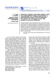
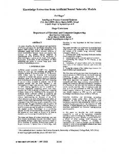
where p∗ is the minimum for estimated prior probabilities (p∗ = #M inority class patterns/#T otal patterns). A priori, it could seem that M S and C objectives could be positively correlated, but while this may be true for small values of M S and C, it is not so for values close to 1 on both M S and C, where the objectives are competitive and conflicting. This fact justifies the use of a MOEA in this research. IV. L EARNING M ETHODOLOGY This paper uses the MOEA described in [30] for training ANN with sigmoid basis functions. The next section briefly explains the schema of this algorithm. For more details about the Base Classifier Framework, Fitness Functions or Local Search Algorithm used, see [30]. A. Memetic Pareto Algorithm The MOEA used is called MPDENN (Memetic Pareto Differential Evolutionary Neural Network). The MPDENN algorithm is based on the PDE algorithm [8] and on the local search algorithm iRprop+ [31]. MPDENN is also based on a previous algorithm described in [32]. In MPDENN, local search does not apply to all offspring to be added to the population. Instead, the most representative offspring of the population are optimized throughout several generations. Fig. 1 shows the framework of the algorithm used in this paper.

III. ACCURACY AND M INIMUM S ENSITIVITY IN C LASSIFICATION P ROBLEMS This section presents two measures to evaluate a classifier: the Correct Classification Rate or Accuracy, and Minimum Sensitivity. To evaluate a classifier, the machine learning community has traditionally used C to measure its default performance. Actually, it suffices to realize that C cannot capture all the different behavioral aspects found in two different classifiers in multiclassification problems. For these problems, two performance measures are considered: traditionally-used C, as the number of patterns correctly classified and the M S in all classes, that is, the lowest percentage of examples correctly predicted as belonging to each class, Si , with respect to the total number of examples in the corresponding class, M S = min{Si } (for a more detailed description of these measures, see [1]). One point in (M S, C) space dominates another if it is above and to the right, i.e. it has greater C and the best M S. Let C and M S be associated with a classifier g, then:

Fig. 1.

Framework for MPDENN.

The MPDENN algorithm starts generating a random population of size M . The population is sorted according to the nondomination concept and dominated individuals are removed from the population. Then the population is adjusted until

M S ≤ C ≤ 1 − (1 − M S)p∗ ,

98

its size is between 3 and half the maximum size by adding dominated individuals or deleting individuals according to their respective distance from their nearest neighbor. After that, the population is completed with new offspring generated from three randomly selected individuals in the population. The child is generated applying the crossover operator to the three parents (α1 , α2 and α3 ). The resultant child is a perturbation of the main parent (α1 ). This perturbation occurs with a probability pc for each neuron. It may be: structural, according to expression (1), where neurons are removed or added to the hidden layer; or parametric, according to expression (2) (for the hidden layer); or (3) (for the output layer), where the weight of the main parent (α1 ) is modified by the difference between the weights of the secondary parents (α2 and α3 ) multiplied by a random variable with normal distribution, N (0, 1). ρchild ← h

�

But, if the number of individuals in the first front is greater than num, a K-means is applied to the first front to get the most representative num individuals, who will then be the object of a local search. The algorithm terminates when the maximum number of generations is reached. B. Proposed Method for Individual Selection The proposed method for individuals selection has two phases. The first phase applies the MPDENN algorithm to obtain a set of individuals, which are sorted in Pareto fronts. The second selects all individuals from the first and second Pareto front. This group of individuals is divided into two subgroups by a 2-means algorithm (because there are two objective functions, C and M S). Next, the two individuals closest to the centroids of clusters are selected, as these are considered the most representative individuals in the population (the fact that these individuals do not have the greatest value in any objective does not mean that they do not generalize well). We decided to include the second Pareto front in the clustering process, in order to expand the number of individuals and to increase diversity. In addition, individuals belonging to this front may have a high percentage of classification in generalization because there is not tend to not over-training in the training phase. In the extreme case there is only one individual in each of the fronts (there would be only two individuals), each of these individuals will be assigned to a cluster.

α2 α3 1 1 if (ρα h +) N (0, 1) (ρh − ρh ) ≥ 0.5 , (1) 0 otherwise

α1 α2 α3 child wih ← wih + N (0, 1) (wih − wih ),

(2)

α1 α2 α3 child who ← who + N (0, 1) (who − who ),

(3)

α2 α3 1 where ρα h , ρh and ρh represent whether or not the hidden α1 neuron h is in the parents α1 , α2 and α3 , respectively; wih is the weight between the input neuron i and hidden neuron α1 is the weight between the hidden h in the parent α1 and who neuron h and output neuron o in the parent α1 . Afterwards, the mutation operator is applied to the child. The mutation operator consists in adding or deleting neurons in the hidden layer depending on a pm probability for each of them. Taking into account the maximum number of hidden neurons that may exist in an individual in a specific problem, the probability is used the same number of times as the number of neurons that are found in the classifier. If the neuron exists, it is deleted, but if it does not exist, then it is created and the weights are established randomly, according to expression (4). � =0 1 if ρchild child h . (4) ← ρh 0 otherwise

V. E XPERIMENTAL S TUDY This section details the experimental study performed using 7 datasets from the UCI repository and 7 methods of selection of individuals from the Pareto front obtained by the MPDENN algorithm. A. Experimental Design The experimental design considers 7 datasets taken from the UCI repository [33]. The design was conducted using a stratified holdout procedure with 30 runs, where approximately 75% of the patterns were randomly selected for the training set and the remaining 25% for the test set. Table I shows the features for each data set.

Finally, the child is added to the population according to dominance relationships with the main parent, that is, the child is added if it dominates the main parent α1 , if there is not dominance relationship with him or if it is the best child of the M rejected children (where M is the population size). In three generations of evolution (the first initially, the second in the middle and the third at the end), the local search algorithm is applied once the population is completed. Local search does not apply to all individuals, only to the most representative. The process for selecting these individuals is as follows: if the number of individuals in the first Pareto front is lower than or equal to the desired number of representative individuals (num), a local search is carried out on all individuals in the first front without needing to apply K-means [10].

TABLE I C HARACTERISTICS FOR THE 7 DATASETS FROM UCI

99

Dataset

#Patterns

#Input variables

#Classes

#Patterns per class

p∗

A. Card Balance Breast-W Ionos Labor Pima Vote

690 625 699 351 57 768 435

51 4 9 34 29 8 16

2 3 2 2 2 2 2

307-383 288-49-288 458-241 126-225 20-37 500-258 267-168

0.4411 0.0641 0.3428 0.3636 0.3571 0.3489 0.3853

In all the experiments, the population size for MPDENN is established at M = 25. The crossover probability is 0.8 and the mutation probability is 0.1. For iRprop+ as local search algorithm, the adopted parameters are η + = 1.2, η − = 0.5, Δ0 = 0.0125 (the initial value of the Δij ), Δmin = 0, Δmax = 50 and Epochs = 5, see [34] for the iRprop+ parameter description.

B. Automatic Methodologies used in the Experimentation Once the Pareto front is built in one run, several strategies or automatic selection methodologies of individuals are used for each run on each problem: •

•

•

•

•

•

MPDENN-E and MPDENN-MS: It consists of choosing the Pareto extreme values in training, that is, the best individual in Entropy (E), because the fitness function of the EA is E, and the best individual in M S. MPDENN-CC (Proposed method): This methodology selects all individuals from the first and second Pareto front (see Section IV-B) provided by fast sorting of nondominated of NSGAII [35]. The individual in training that is chosen is the one closest to the centroids of clusters obtained, taking the C measure into account. MPDENN-CMS (Proposed method): This automatic methodology chooses in a similar way to the MPDENNCC automatic methodology, but in this case, the individual obtained closest to the centroids of clusters is selected taking the M S measure into account. MPDENN-MV: With this technique, a pattern belong to the class that has the most votes, according to the independent classification of each of the elements that make up the ensemble. To estimate the a posteriori probability of a pattern to belong to a class, the average of the output probabilities of the models who voted for this class are used. This is performed for each pattern in the training of generalization dataset so that a probability matrix is formed to obtain the RM SE measure. MPDENN-SA: This technique calculates for each pattern the arithmetic mean of the probability of assignment to each Q class for each of the models in the ensemble. The assignment will take the class that has the highest average probability. For the case of the RM SE measure, the arithmetic mean of the probabilities (using softmax function) is obtained for each output of each model in the ensemble for a particular pattern. Then we use the probabilities of the output with the maximum mean probability for each model of the ensemble for that particular pattern. This is done for each pattern in the training and generalization dataset, and a probability matrix is formed to obtain the RM SE measure. MPDENN-WT: With this ensemble method, for each pattern the probabilities of the model with the highest probability in one of the outputs are used as the output of the ensemble.

VI. R ESULTS Table II presents the values of mean and Standard Deviation (SD) for C, M S, RM SE and Cohen’s KAP P A in generalization in 30 runs of all the experiments performed. The analysis of the results leads us to conclude that the MPDENN-CC obtained the best performance for five datasets and MPDENN-CMS for two datasets considering CG . For M SG , the MPDENN-MS obtained the best results for four datasets and the MPDENN-CC and MPDENN-E yielded the highest performance for three an two datasets respectively (note that the Labor dataset produces many ties in all metrics, because the first Pareto front has a unique individual). The MPDENN-CC got the best results for RM SEG for four datasets. For KAP P AG , the MPDENN-CC, MPDENNCMS and MPDENN-E obtained the best performance for two datasets each one and MPDENN-WT in the remaining dataset. Table III shows the mean values for all metrics over all datasets and the mean ranking of each of the methods. From a descriptive point of view, we can consider that the best method for CG , RM SEG and KAP P AG is the MPDENN-CC while it is MPDENN-MS for M SG , because their mean ranking are lower. A performance analysis of the results using parametric statistical treatment could lead to mistaken conclusions, since a previous evaluation of the CG , M SG , RM SEG and KAP P AG value resulted in rejecting the normality and the equality of the variance hypothesis. Therefore, in order to determine the statistical significance of the rank differences observed for each method in the different datasets, three non-parametric Friedman tests [36] have been carried out with the ranking of CG , M SG , RM SEG and KAP P AG of the best models as the test variables. These tests show that the effect of the method used for classification is statistically significant at a significance level of 5% for CG , M SG , RM SEG and KAP P AG , as the confidence interval is C0 = (0, F0.05 = 2.36) and the F-distribution statistical values are F ∗ = 6.14 ∈ / C0 for CG , F ∗ = 3.02 ∈ / C0 for M SG , F ∗ = 1.88 ∈ C0 for RM SEG and F ∗ = 1.89 ∈ C0 for KAP P AG . Consequently, we reject the null-hypothesis stating that all algorithms perform equally in mean ranking of CG and M SG and we accept it for RM SEG and KAP P AG . As there are significant differences in CG and M SG , two post-hoc statistical analyses were required. These analyses chose the best performing model as the control method for comparison with the rest of the methods (MPDENN-CC for CG and MPDENN-MS for M SG ). Based on the rejection of the Friedman tests, the BonferroniDunn test is used to compare all classifier to each other. This test considers that the performance of any two classifiers is deemed to be significantly different if their mean ranks differ by at least the critical difference (CD): � K(K + 1) , CD = q 6D where K is the number of classifiers, D the number of datasets and the q value can be computed as suggested in [37]. Fig.

100

TABLE II S TATISTICAL RESULTS FOR DIFFERENT METHODS IN GENERALIZATION CG (%) Mean±SD

Dataset

Methodology

A. Card

MPDENN-E MPDENN-MS MPDENN-CC MPDENN-CMS MPDENN-MV MPDENN-SA MPDENN-WT

86.26 86.28 86.47 86.28 85.59 85.82 86.47

Balance

MPDENN-E MPDENN-MS MPDENN-CC MPDENN-CMS MPDENN-MV MPDENN-SA MPDENN-WT

90.88 91.47 91.71 92.12 48.55 91.56 91.79

BreastW

MPDENN-E MPDENN-MS MPDENN-CC MPDENN-CMS MPDENN-MV MPDENN-SA MPDENN-WT

95.22 95.16 95.33 94.97 94.82 94.93 94.86

Ionos

MPDENN-E MPDENN-MS MPDENN-CC MPDENN-CMS MPDENN-MV MPDENN-SA MPDENN-WT

92.61 92.88 92.73 92.92 91.17 91.33 91.44

Labor

MPDENN-E MPDENN-MS MPDENN-CC MPDENN-CMS MPDENN-MV MPDENN-SA MPDENN-WT

82.14 82.14 83.10 82.38 82.14 82.14 82.14

Pima

MPDENN-E MPDENN-MS MPDENN-CC MPDENN-CMS MPDENN-MV MPDENN-SA MPDENN-WT

78.75 76.48 78.83 76.94 75.89 77.12 77.93

Vote

M SG (%) Mean±SD

± ± ± ± ± ± ±

1.49 1.72 1.34 1.65 1.83 1.97 1.97

84.67 85.17 85.18 85.00 84.89 84.64 84.65

± ± ± ± ± ± ±

1.36 1.22 1.13 1.72 1.26 0.95 0.78

± ± ± ± ± ± ±

0.83 0.83 0.86 0.83 0.96 0.90 0.93

± ± ± ± ± ± ±

± ± ± ± ± ± ± ± ± ± ± ± ± ±

RM SEG Mean±SD

± ± ± ± ± ± ±

2.15 1.98 1.74 1.97 2.25 2.54 2.36

0.3215 0.3225 0.3210 0.3239 0.3231 0.3229 0.3256

28.67 ± 17.56 86.81 ± 5.29 33.00 ± 13.17 74.80 ± 14.48 1.19 ± 1.23 68.73 ± 12.63 80.42 ± 11.24

0.1931 0.2101 0.1921 0.1970 0.1957 0.1950 0.1924

2.43 2.47 2.40 2.25 2.20 2.21 2.37

0.1897 0.1905 0.1930 0.1945 0.1982 0.1980 0.1994

2.10 2.15 1.81 1.76 2.47 2.45 2.58

83.02 84.06 83.33 83.85 81.04 80.73 81.52

± ± ± ± ± ± ±

5.73 5.82 4.37 4.27 6.46 6.72 6.92

0.2486 0.2452 0.2440 0.2436 0.2745 0.2735 0.2748

9.14 9.14 8.28 7.90 9.14 9.14 9.14

70.44 70.44 64.89 64.81 70.44 70.44 70.44

15.40 15.40 14.89 14.82 15.40 15.40 15.40

0.3705 0.3705 0.3732 0.3731 0.3705 0.3705 0.3705

1.69 1.69 2.08 2.65 2.37 1.84 1.97

62.34 72.31 63.93 70.27 67.11 67.81 58.16

± ± ± ± ± ± ±

4.36 3.48 5.32 5.35 4.34 3.89 6.24

0.3909 0.3962 0.3904 0.3934 0.3925 0.3912 0.3975

90.44 90.22 89.50 89.39 88.89 89.00 88.50

± ± ± ± ± ± ±

± ± ± ± ± ± ±

MPDENN-E 93.21 ± 1.44 90.63 ± 2.79 MPDENN-MS 93.21 ± 1.48 90.71 ± 2.89 MPDENN-CC 93.67 ± 1.33 91.03 ± 2.19 MPDENN-CMS 93.43 ± 1.23 90.61 ± 2.38 MPDENN-MV 93.27 ± 1.66 90.40 ± 3.28 MPDENN-SA 93.39 ± 1.59 90.36 ± 3.34 MPDENN-WT 93.36 ± 1.57 90.16 ± 3.35 The best result is in bold face and the second

101

KAP P AG Mean±SD

± ± ± ± ± ± ±

0.0130 0.0147 0.0110 0.0124 0.0136 0.0134 0.0154

0.7222 0.7229 0.7267 0.7231 0.7169 0.7138 0.7280

± ± ± ± ± ± ±

0.0061 0.0113 0.0077 0.0090 0.0050 0.0049 0.0073

0.8335 0.8538 0.8490 0.8622 0.1116 0.8518 0.8580

± ± ± ± ± ± ±

0.0155 0.0144 0.0160 0.0164 0.0143 0.0142 0.0155

0.8925 0.8911 0.8879 0.8866 0.8859 0.8855 0.8836

± ± ± ± ± ± ±

0.0298 0.0304 0.0226 0.0235 0.0377 0.0374 0.0386

0.8351 0.8414 0.8380 0.8424 0.8085 0.8058 0.8089

0.0761 0.0761 0.0754 0.0702 0.0761 0.0761 0.0761

0.6027 0.6027 0.6111 0.5966 0.6027 0.6027 0.6027

± ± ± ± ± ± ±

0.0054 0.0085 0.0085 0.0113 0.0100 0.0095 0.0124

0.5161 0.4963 0.5076 0.5003 0.4960 0.4977 0.4896

± ± ± ± ± ± ±

0.2370 ± 0.0228 0.2376 ± 0.0238 0.2277 ± 0.0209 0.2315 ± 0.0182 0.2308 ± 0.0217 0.2306 ± 0.0215 0.2314 ± 0.0217 best result in italics.

0.8563 0.8564 0.8662 0.8609 0.8599 0.8599 0.8592

± ± ± ± ± ± ±

0.0305 0.0348 0.0271 0.0333 0.0363 0.0397 0.0393

± ± ± ± ± ± ±

0.0190 0.0191 0.0199 0.0189 0.0218 0.0206 0.0214

± ± ± ± ± ± ±

0.2066 0.2066 0.1927 0.1839 0.2066 0.2066 0.2066

± ± ± ± ± ± ±

0.0307 0.0316 0.0279 0.0263 0.0333 0.0341 0.0338

± ± ± ± ± ± ±

± ± ± ± ± ± ±

± ± ± ± ± ± ±

0.0258 0.0204 0.0205 0.0298 0.0221 0.0171 0.0135

0.0489 0.0502 0.0410 0.0399 0.0564 0.0573 0.0597

0.0376 0.0379 0.0478 0.0596 0.0381 0.0410 0.0507

M EAN

TABLE III VALUES OF ALL METRICS OVER ALL DATASETS IN GENERALIZATION AND MEAN RANKING

MPDENN-E

MPDENN-MS

MPDENN-CC

MPDENN-CMS

MPDENN-MV

MPDENN-SA

MPDENN-WT

C G (%) R CG

88.43 4.35

88.23 4.42

88.83 1.64

88.43 2.64

81.63 6.42

88.04 4.71

88.28 3.78

M S G (%) RM SG

72.88 4.00

82.81 1.71

72.98 3.42

79.81 3.57

69.13 5.0

78.81 5.0

79.12 5.28

RM SE G RRM SEG

0.2787 3.00

0.2818 4.42

0.2773 2.28

0.2795 4.71

0.2836 4.57

0.2831 3.71

0.2845 5.28

KAP P AG RKAP P AG

0.7512 4.00

0.7520 0.7552 0.7531 0.6402 3.71 2.42 3.00 5.35 The best result is in bold face and the second best result in italics.

0.7453 5.07

0.7471 4.42

TABLE IV A DJUSTED p- VALUES

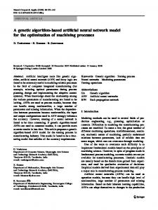
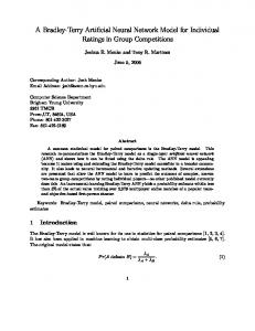
2 shows the application of the Bonferroni-Dunn test for each test variable. This graph is a bar chart where the bars have a height proportional to the mean ranking obtained for each algorithm, following the procedure of Friedman. Adding the ranking value of the lowest bar (associated with the MPDENNCC method in CG and MPDENN-MS in M SG ) to the CD value, a vertical line is obtained (denoted as “Threshold”), which is displayed in the graph. The bars exceeding this line are those associated with the methods whose performance is significantly worse than the control method. The CG threshold is 4.68 and M SG threshold is 4.75 for α = 0.05. From the results of these tests, it can be concluded that the MPDENN-CC (control method for CG ) produced a significantly better CG ranking than MPDENN-MV and MPDENN-SA and that the MPDENN-MS (control method for M SG ) obtained significant differences in M SG compared to MPDENN-MV, MPDENNSA and MPDENN-WT.

Variable test: CG Control method: MPDENN-CC algorithm

unadjusted p

pBonf

pHolm

pHochberg

MPDENN-E MPDENN-MS MPDENN-CMS MPDENN-MV MPDENN-SA MPDENN-WT

0.0187 0.0158 0.3864 3.40 · 10−5 0.0078 0.0634

0.1124 0.0950 2.3188 2.04 · 10−4 0.0468 0.3809

0.0633 0.0633 0.3864 2.04 · 10−4 0.0390 0.1269

0.0562 0.0562 0.3864 2.04 · 10−4 0.0390 0.1269

Variable test: M SG Control method: MPDENN-MS algorithm

unadjusted p

pBonf

pHolm

pHochberg

MPDENN-E MPDENN-CC MPDENN-CMS MPDENN-MV MPDENN-SA MPDENN-WT

0.0477 0.1376 0.1077 0.0044 0.0044 0.0019

0.2865 0.8258 0.6465 0.0266 0.0266 0.0118

0.1432 0.2155 0.2155 0.0221 0.0221 0.0118

0.1376 0.1376 0.1376 0.0177 0.0177 0.0118

of a hypothesis that results in a rejection. This provides a way to know whether two methods are significantly different and also a metric to show how different they are. The results of these tests indicate that there are significant differences as determined by the Bonferroni-Dunn test. VII. C ONCLUSION

Fig. 2.

Bonferroni-Dunn graphic for α = 0.05.

More powerful tests, such as Holm’s and Hochberg’s tests [37], were used to compar the control method (MPDENNCC for CG and MPDENN-MS for M SG ) with the rest of the models. Table IV shows all the adjusted p-values for each comparison, using CG and M SG as the test variables. The adjusted p-values represent the lowest level of significance

The present work studies the use of different techniques for selecting Artificial Neural Networks in the Pareto front in classification problems where Accuracy is the measure considered to evaluate classifier performance along with the Minimum Sensitivity measure. Minimum Sensitivity is used to avoid the design of classifiers with high global performance but bad performance when considering the classification rate for each class, very frequently problem in imbalanced dataset. Experimentally it has been proven that the MPDENN-CC technique improves classifier accuracy. Furthermore, taking into account the Minimum Sensitivity measure, the MPDENNMS technique achieved the best mean Minimum Sensitivity value and the best Minimum Sensitivity mean ranking. Finally, the methodologies proposed for the selection of classifiers based on the application of the K-means algorithm over the

102

Pareto front achieved, in general, a better significant mean ranking than the standard ensemble techniques considered in the literature (Majority Voting, Simple Averaging and Winner Take All). As a future work and in order to make the conclusions more robust, it would be interesting to extend the experimental study with more datasets. Especially it would be suitable to study the result in multiclass and imbalanced problems, since in them the Accuracy and Minimum Sensitivity measures are more in conflict. In addition, the proposed method could be compared with some state-of-the-art ensemble neural network classification method or multi-class classification methods to highlight the efficacy of the proposed scheme. ACKNOWLEDGMENT This work has been partially subsidized by the TIN 200806681-C06-03 project of the Spanish Ministerial Commission of Science and Technology (MICYT), FEDER funds and the P08-TIC-3745 project of the “Junta de Andaluc´ıa” (Spain). M. Cruz-Ram´ırez’s research has been subsidized by the FPU Predoctoral Program (Spanish Ministry of Education and Science), grant reference AP2009-0487.Francisco Fern´andezNavarro’s research has been funded by the “Junta de Andaluc´ıa” Predoctoral Program, grant reference P08-TIC-3745. Javier S´anchez-Monedero’s research has been funded by the “Junta de Andaluc´ıa” Ph. D. Student Program. R EFERENCES [1] J. C. Fern´andez-Caballero, F. J. Mart´ınez-Estudillo, C. Herv´as-Mart´ınez, and P. A. Guti´errez, “Sensitivity versus accuracy in multiclass problems using memetic Pareto evolutionary neural networks,” IEEE Transactions on Neural Networks, vol. 21, no. 5, pp. 750 –770, may 2010. [2] J. C. Fern´andez-Caballero, C. Herv´as-Mart´ınez, F. J. Mart´ınez-Estudillo, and P. A. Guti´errez, “Memetic Pareto Evolutionary Artificial Neural Networks to determine growth/no-growth in predictive microbiology,” Applied Soft Computing, vol. 11, no. 1, pp. 534 – 550, 2011. [3] T. L¨ofstr¨om, U. Johansson, and H. Bostr¨om, “Ensemble member selection using multi-objective optimization,” in IEEE Symposium on Computational Intelligence and Data Mining, 2009, pp. 245–251. [4] G. P. Zhang, “Neural networks for classification: A survey,” IEEE Transactions on Systems, Man and Cybernetics, Part C: Applications and Reviews, vol. 30, no. 4, pp. 451–462, 2000. [5] V. Pareto, Cours D’Economie Politique. Lausanne: F. Rouge, 1886, vol. 1 and 2. [6] R. Storn, Differential evolution research - Trends and open questions, 2008, vol. 143. [7] J. Ilonen, J. Kamarainen, and J. Lampinen, “Differential evolution training algorithm for feed-forward neural networks,” Neural Processing Letters, vol. 17, pp. 93–105, 2003. [8] H. A. Abbass, R. Sarker, and C. Newton, “PDE: a Pareto-frontier differential evolution approach for multi-objective optimization problems,” in Proceedings of the 2001 Congress on Evolutionary Computation, vol. 2, Seoul, South Korea, 2001. [9] M. Bhuiyan, “An algorithm for determining neural network architecture using differential evolution,” 2009, pp. 3–7. [10] J. MacQueen, “Some methods for classification and analysis of multivariate observations,” in Proc. of the 5th Berkeley Symposium on Mathematical Statistics and Probability. U. C. Berkeley Press, 1967, pp. 281–297. [11] L. Rokach, “Taxonomy for characterizing ensemble methods in classification tasks: A review and annotated bibliography,” Computational Statistics and Data Analysis, vol. 53, no. 12, pp. 4046–4072, 2009. [12] G. Brown, J. Wyatt, R. Harris, and X. Yao, “Diversity creation methods: A survey and categorisation,” Inf. Fusion, vol. 6, no. 1, pp. 5–20, 2005.

[13] S. Theodoridis and K. Koutroumbas, Pattern Recognition, 3rd ed. Elsevier, Academic Press, 2006. [14] A. Chandra and X. Yao, “Ensemble learning using multi-objective evolutionary algorithms,” Journal of Mathematical Modelling and Algorithms, vol. 5, no. 4, pp. 417–445, 2006. [15] ——, “Divace: Diverse and accurate ensemble learning algorithm,” in Proceedings of the Fifth International Conference on intelligent Data Engineering and Automated learning, vol. 3177. Exeter, UK: Lectures Notes and Computer Science, Springer, Berlin, 2004, pp. 619–625. [16] Y. Liu, X. Yao, and T. Higuchi, “Ensembles with negative correlation learning,” IEEE Transactions on Evolutionary Computation, vol. 4, no. 4, pp. 380–387, 2000. [17] H. A. Abbass, “Pareto Neuro-Evolution: Constructing Ensemble of Neural Networks Using Multi-objective Optimization,” in Proceedings of the 2003 Congress on Evolutionary Computation (CEC’2003), vol. 3. Canberra, Australia: IEEE Press, 2003, pp. 2074–2080. [18] M. Islam and X. Yao, “A constructive algorithm for training cooperative neural networks ensembles,” IEEE transactions on Neural Networks, vol. 14, no. 4, pp. 820–834, 2003. [19] Y. Liu and X. Yao, “Ensemble learning via negative correlation,” Neural Networks, vol. 12, no. 10, pp. 1399–1404, 1999. [20] N. Garc´ıa-Pedrajas, C. Herv´as-Mart´ınez, and D. Ortiz-Boyer, “Cooperative coevolution of artificial neural network ensembles for pattern classification,” IEEE Transactions on Evolutionary Computation, vol. 9, no. 3, pp. 271–302, 2005. [21] D. Opitz and R. Maclin, “Popular ensemble methods: An empirical study,” J. of Artificial Intelligence Research, vol. 11, pp. 169–198, 1999. [22] H. Chen and X. Yao, “Regularized negative correlation learning for neural network ensembles,” IEEE Transactions on Neural Networks, vol. 20, no. 12, pp. 1962–1979, 2009. [23] ——, “Multi-objective neural network ensembles based on regularized negative correlation learning,” IEEE Transactions on Knowledge and Data Engineering, p. In Press, 2009. [24] F. L. Minku and T. B. Ludemir, “Clustering and co-evolution to construct neural network ensembles: An experimental study,” Neural Networks, vol. 21, pp. 1363–1379, 2008. [25] R. Storn and K. Price, “Differential evolution. a fast and efficient heuristic for global optimization over continuous spaces,” Journal of Global Optimization, vol. 11, pp. 341–359, 1997. [26] Y. Jin and B. Sendhoff, “Pareto-based multiobjective machine learning: An overview and case studies,” IEEE Trans. Syst., Man, Cybern. Part C: Applications and Reviews, vol. 38, no. 3, pp. 397–415, 2008. [27] H. Abbass, “An evolutionary artificial neural networks approach for breast cancer diagnosis,” Artificial Intelligence in Medicine, vol. 25, no. 3, pp. 265–281, 2002. [28] K. V. Price, R. M. Storn, and J. . A. Lampinen, Differential Evolution. A Practical Approach to Global Optimization, ser. Natural Computing Series. Springer, 2005. [29] U. K. Chakraborty, Advances in Differential Evolution. Springer, 2008. [30] M. Cruz-Ram´ırez, J. S´anchez-Monedero, F. Fern´andez-Navarro, J. Fern´andez, and C. Herv´as-Mart´ınez, “Memetic pareto differential evolutionary artificial neural networks to determine growth multi-classes in predictive microbiology,” Evolutionary Intelligence, vol. 3, no. 3-4, pp. 187–199, 2010. [31] C. Igel and M. H¨usken, “Improving the rprop learning algorithm,” Proc. Proceedings of the Second International ICSC Symposium on Neural Computation (NC 2000), ICSC Academic Press, pp. 115–121, 2000. [32] J. C. Fern´andez, C. Herv´as, F. J. Mart´ınez, P. A. Guti´errez, and M. Cruz, “Memetic Pareto differential evolution for designing artificial neural networks in multiclassification problems using cross-entropy versus sensitivity,” in Hybrid Artificial Intelligence Systems, vol. 5572. Springer Berlin / Heidelberg, 2009, pp. 433–441. [33] A. Asuncion and D. Newman, “UCI machine learning repository,” 2007. [Online]. Available: http://www.ics.uci.edu/ mlearn/MLRepository.html [34] C. Igel and M. H¨usken, “Empirical evaluation of the improved rprop learning algorithms,” Neurocomputing, vol. 50, no. 6, pp. 105–123, 2003. [35] K. Deb, A. Pratab, S. Agarwal, and T. Meyarivan, “A fast and elitist multiobjective genetic algorithm: Nsga2,” IEEE Transactions on Evolutionary Computation, vol. 6, no. 2, pp. 182–197, 2002. [36] M. Friedman, “A comparison of alternative tests of significance for the problem of m rankings,” Annals of Mathematical Statistics, vol. 11, no. 1, pp. 86–92, 1940. [37] Y. Hochberg and A. Tamhane, Multiple Comparison Procedures. John Wiley & Sons, 1987.

103