Selecting the optimal method to calculate daily global reference ...

Hydrol. Earth Syst. Sci., 16, 983–1000, 2012 www.hydrol-earth-syst-sci.net/16/983/2012/ doi:10.5194/hess-16-983-2012 © Author(s) 2012. CC Attribution 3.0 License.

Hydrology and Earth System Sciences

Selecting the optimal method to calculate daily global reference potential evaporation from CFSR reanalysis data for application in a hydrological model study ¨ 1 , M. Vrac4 , and L. P. H. van Beek1 F. C. Sperna Weiland1,2 , C. Tisseuil3 , H. H. Durr 1 Department

of Physical Geography, Utrecht University, P.O. Box 80115, 3508 TC, Utrecht, The Netherlands P.O. Box 177, 2600 MH, Delft, The Netherlands 3 Mus´ eum National d’Histoire Naturelle, UMR BOREA-IRD 207/CNRS 7208/MNHN/UPMC, D´epartement Milieux et Peuplements Aquatiques, Paris, France 4 Laboratoire des Sciences du Climat et de l’Environnement (LSCE-IPSL) CNRS/CEA/UVSQ, Centre d’´ etude de Saclay, Orme des Merisiers, 91191 Gif-sur-Yvette Cedex, France 2 Deltares,

Correspondence to: F. C. Sperna Weiland ([email protected]) Received: 1 July 2011 – Published in Hydrol. Earth Syst. Sci. Discuss.: 28 July 2011 Revised: 15 March 2012 – Accepted: 16 March 2012 – Published: 27 March 2012

Abstract. Potential evaporation (PET) is one of the main inputs of hydrological models. Yet, there is limited consensus on which PET equation is most applicable in hydrological climate impact assessments. In this study six different methods to derive global scale reference PET daily time series from Climate Forecast System Reanalysis (CFSR) data are compared: Penman-Monteith, Priestley-Taylor and original and re-calibrated versions of the Hargreaves and BlaneyCriddle method. The calculated PET time series are (1) evaluated against global monthly Penman-Monteith PET time series calculated from CRU data and (2) tested on their usability for modeling of global discharge cycles. A major finding is that for part of the investigated basins the selection of a PET method may have only a minor influence on the resulting river flow. Within the hydrological model used in this study the bias related to the PET method tends to decrease while going from PET, AET and runoff to discharge calculations. However, the performance of individual PET methods appears to be spatially variable, which stresses the necessity to select the most accurate and spatially stable PET method. The lowest root mean squared differences and the least significant deviations (95 % significance level) between monthly CFSR derived PET time series and CRU derived PET were obtained for a cell-specific recalibrated Blaney-Criddle equation. However, results show that this re-calibrated form is likely to be unstable under changing climate conditions and less reliable for the calculation of daily time series. Although often recommended, the Penman-Monteith equation applied to the CFSR data did not outperform the other methods in a evaluation against PET

derived with the Penman-Monteith equation from CRU data. In arid regions (e.g. Sahara, central Australia, US deserts), the equation resulted in relatively low PET values and, consequently, led to relatively high discharge values for dry basins (e.g. Orange, Murray and Zambezi). Furthermore, the Penman-Monteith equation has a high data demand and the equation is sensitive to input data inaccuracy. Therefore, we recommend the re-calibrated form of the Hargreaves equation which globally gave reference PET values comparable to CRU derived values for multiple climate conditions. The resulting gridded daily PET time series provide a new reference dataset that can be used for future hydrological impact assessments in further research, or more specifically, for the statistical downscaling of daily PET derived from raw GCM data. The dataset can be downloaded from http://opendap.deltares.nl/thredds/dodsC/ opendap/deltares/FEWS-IPCC.

1

Introduction

Climate change is likely to induce alterations in the hydrological cycle (IPCC, 2007 and references therein). To assess and quantify the possible changes, multiple hydrological impact studies have been conducted on the local, continental and global scale, the latter being of interest in this study. In addition to temperature and precipitation (PR; for list of abbreviations see Table 1), evaporation is required as input for most hydrological models used in impact studies (Kay and Davies, 2008; Oudin et al., 2005). However, both potential

Published by Copernicus Publications on behalf of the European Geosciences Union.

984

F. C. Sperna Weiland et al.: Calculating global potential evaporation from CFSR re-analysis data

and actual evapotranspiration (AET; for list of abbreviations see Table 1) are seldomly monitored and General Circulation Model (GCM) datasets, employed for future impact assessments (Sperna Weiland et al., 2012b), often lack AET data (PCMDI, 2010). Here, we prefer to calculate potential evaporation (PET) from GCM data and to derive AET within a hydrological model over using GCM AET directly. This because within global hydrological models (GHMs), AET is calculated on a higher grid resolution and processes related to transpiration and soil moisture are modeled with a water balance instead of energy balance approach which at least guarantees that negative evaporation does not occur (Sperna Weiland et al., 2012a). In addition, GCM AET is often biased due to, amongst others, biases in PR, radiation and soil moisture availability (Mahanama and Koster, 2005; Elshamy et al., 2009; Sperna Weiland et al., 2012a). Of course, it should be noted here that off-line calculation of PET and AET can also be biased by deviations in GCM radiation used as input for some of the PET equations or through interaction between the different atmospheric variables within the GCM. Within hydrological model studies monthly PET timeseries, or monthly PET time-series downscaled to daily values (for example based on temperature), have frequently been used (Van Beek, 2008; Sperna Weiland et al., 2010; Arnell, 2011). Currently, most hydrological models run on a daily or smaller time-step, as most hydrological processes show a high variability over time. Consequently, these models can also benefit from daily PET time-series as model input. In addition, the input data of PET equations is now often provided on a daily time step. Therefore, this study focuses on calculation of daily PET time series using daily values of the required atmospheric variables. A historical global gridded PET time series will be created that can be used as reference for the statistical downscaling of daily GCM data. Downscaling of PET time series was preferred over downscaling of the individual GCM input variables of the PET equation, since by individual downscaling inconsistencies between the atmospheric input variables can be introduced (Piani et al., 2010). For the creation of these PET time series a consistent observational dataset of current climatic conditions at high spatial and temporal resolution is needed. Here we used the recently developed Climate Forecast System Reanalysis (CFSR) dataset (Saha et al., 2006, 2010) which is of particular interest for three major reasons. Firstly, it is a data set with a high spatial (∼0.3◦ × ∼0.3◦ ) and temporal (6-hourly) resolution covering the entire globe. Secondly, in the short term, the CFSR dataset is likely to supersede its predecessor, the widely known US NCEP/NCAR (National Center for Environmental Prediction/National Center for Atmospheric Research) reanalysis data (Kalnay et al., 1996). And thirdly, the CFSR dataset contains all required atmospheric fields to calculate and compare a range of PET equations.

Hydrol. Earth Syst. Sci., 16, 983–1000, 2012

Table 1. Abbreviations. Abbreviaton

Long name/description

AET BC BCorig BCrecal CDF CFSR CFSR PET CFSR PM PET CRU CRU TS 2.1 CRU CL 1.0 CRU PET CRU PM PET CV DJF FAO GCM GHM GLCC GRDC HG HGorig HGrecal HGPET JJA MAM NCAR NCEP PCR-GLOBWB PET PM PR PT QC QL RMSD SON US

Actual evapotranspiration Blaney-Criddle Original Blaney-Criddle equation Re-calibrated Blaney-Criddle equation Cumulative distribution function Climate forecast system reanalysis Potential evaporation calculated from CFSR data Penman-Monteith potential evaporation from CFSR data Climate research unit, University of East Anglia 1901–96 Monthly Grids of Terrestrial Surface Climate, CRU 1961-90 mean monthly terrestrial climatology, CRU Potential evaporation calculated from CRU data Penman-Monteith potential evaporation from CRU data Coefficient of variation December, January, February United Nations Food and Agriculture Organization General circulation model / global climate model Global hydrological model Global Land Cover Characterization Global runoff data centre Hargreaves equation Original Hargreaves equation Re-calibrated Hargreaves equation Hargreaves potential evaporation June, July, August March, April, May National Center for Atmospheric Research National Centre for Environmental Prediction PCRaster code global water balance model Potential evaporation Penman-Monteith Precipitation Priestley-Taylor (Channel) discharge Cell specific runoff Root mean squared difference September, October, November United States

Limited consensus exists on which PET equation is most applicable in global hydrological impact studies. Several studies illustrated that the selected method can actually determine the direction of projected change in future water availability (Boorman, 2010; Kingston et al., 2009; Arnell, 1999). Therefore, we here analyze six well documented equations of different complexity: the physical-based Penman-Monteith equation (PM), the empirical Hargreaves (HG), PriestleyTaylor (PT) and Blaney-Criddle (BC) equations and modified versions of the Hargreaves (HGrecal) and Blaney-Criddle (BCrecal) equations. The PM equation is generally considered as the standard (Hargreaves et al., 2003; Droogers and Allen, 2002; Gavil´an et al., 2006) as its physically based nature is preferred over simpler empirical equations (Kay and Davies, 2008; Arnell, 1999; Kingston et al., 2009). However, due to its high input data requirement the PM may be sensitive to biases in mulptiple GCM and re-analysis atmospheric variables (Oudin et al., 2005). The HG equation is a simplified alternative for the PM equation (Hargreaves and Samani, 1985; Hargreaves et al., 2003). Here the influence of humidity is approximated with the diurnal temperature range. www.hydrol-earth-syst-sci.net/16/983/2012/

F. C. Sperna Weiland et al.: Calculating global potential evaporation from CFSR re-analysis data The equation is applicable in a variety of climatic conditions and shows overall good agreement with the PM method (Droogers and Allen, 2002). Several studies highlighted significant improvement of the HG equation by increasing its multiplication factor (Droogers and Allen, 2002). This will be tested here as well. The more empirical BC equation depends on less input variables and may therefore be less sensitive to GCM and reanalysis data quality (Kingston et al., 2009; Weiß and Menzel, 2008; Lu et al., 2005). With the temperature-based BC equation the computation time required for both calculation of PET and downscaling of the required input variables can be reduced, while the method provides results comparable to other PET methods (Oudin et al., 2005; Blaney and Criddle, 1950). Yet, Jensen (1966) showed that the climate dependency of the BC equation disables its application in multiple different climate zones. To overcome this problem we tested the local-recalibrated BC method proposed by Ekstr¨om et al. (2007). The main goal of this study is the construction of a global gridded dataset of reference PET at high spatial (0.5 degree) and temporal (daily) resolution from CFSR reanalysis data using one of the following six PET equations; PM, HG, PT, BC and the HGrecal and BCrecal equations. The constructed daily PET dataset will be validated annually and seasonally for the period 1979–2002 against the Climate Research Unit (CRU) dataset (CRU TS 2.1 and CRU CL 1.0) which is often considered as a standard (Mitchell and Jones, 2005; New et al., 2000, 1999; Droogers and Allen, 2002; IPCC, 2007). In a first step, a sensitivity analysis of the influence of the differences between individual CFSR and CRU atmospheric variables on calculated PET is given. In a final step, the transfer of differences between the six PET methods throughout the hydrological modeling chain (i.e. from PET to AET to runoff and discharge) will be assessed by inter-method comparison and the goodness-of-fit between modeled and observed river discharge.

2 2.1

Data and methods CFSR reanalysis data

The CFSR dataset is a reanalysis product which is developed as part of the Climate Forecast System (Saha et al., 2006, 2010) at the National Centers for Environmental Prediction (NCEP). The CFSR dataset became available in 2010 and supersedes the previous NCEP/NCAR reanalysis dataset which has been widely used in downscaling studies (e.g. Michelangeli et al., 2009; Maurer et al., 2010; Wilby et al., 1998). At this stage the CFSR dataset spans the period 1979 to present and has a resolution of approximately 0.25 degrees around the equator to 0.5 degrees beyond the tropics (Higgins et al., 2010). In this study, 6-hourly temperature, radiation, air pressure and wind data were averaged to a daily time-step for www.hydrol-earth-syst-sci.net/16/983/2012/

985

the period 1979–2002. These daily time series were then interpolated to the regular 0.5 degrees PCR-GLOBWB model grid using bilinear interpolation. 2.2

CRU reference potential evaporation

For validation reference historical PET time series were calculated from the CRU datasets with the by the United Nations Food and Agriculture Organization (FAO) recommended PM equation (Monteith, 1965; Allen et al., 1998). Temperature, vapor pressure and cloud cover were retrieved from the CRU TS2.1 monthly time series (New et al., 2000). Wind speed was obtained from the monthly climatology, CRU CL 1.0 (New et al., 1999) because monthly CRU TS2.1 time series are not provided for this variable. Diffusivity, i.e. the effectiveness by which heat and vapour can be exchanged with the atmosphere, was calculated following Allen et al. (1998). As radiation is not included in the CRU datasets, a standard climatological maximum radiation cycle was calculated using the day-number and latitude as input (Allen et al., 1998). This maximum radiation was reduced to incoming radiation at the surface with monthly CRU cloud cover time-series. The resulting monthly PET time series, which are here used as reference for the validation of the CFSR derived PET, are subject to uncertainties as well due to biases in and availability of the meteorological input data and due to simplifications in the equation. Yet, to our opinion they form one of the best available global reference PET dataset (Mitchell and Jones, 2005; Droogers and Allen, 2002; IPCC, 2007). For application in the hydrological model the CRU time-series have been downscaled to daily values using the monthly PR and temperature quantities from the CRU datasets and the daily distribution of these variables from the CFSR dataset following Van Beek et al. (2008). It should be noted that the measurement based CRU dataset is subject to inaccuracies as well. In addition, the data from the CRU CL 1.0 climatology is derived from data for the period 1961 to1990 and has been used for the calculation of PET for the period 1990 to 2002 as well. This may have introduced inconsistencies due to meteorological changes over the past decades. The influence of these inconsistencies is minimized by analyzing long-term average PET results only. 2.3

Potential evaporation equations

Within this study we compare daily CFSR PET time series derived with six different PET equations. The equations considered are: (1) the physically based PM equation, (2) the radiation and temperature-based PT equation, (3) the HG equation which requires as input time-varying temperature and extra-terrestrial radiation, (4) the empirical temperaturebased BC equation and additional modified forms of the (5) HG and (6) BC equations (Table 2). The BC equation was applied in its original form (BCorig) and in a re-calibrated form (BCrecal) following Ekstr¨om et Hydrol. Earth Syst. Sci., 16, 983–1000, 2012

986

F. C. Sperna Weiland et al.: Calculating global potential evaporation from CFSR re-analysis data

Table 2. Potential evaporation equations. Method

Acronym

Equation

Penman-Monteith

PM

ET0 =

HGorig HGrecal PT BCorig BCrecal

ET0 = 0.0023 · Ra · (T + 17.8) · TR0.50 ET0 = 0.0031 · Ra · (T + 17.8) · TR0.50 1Rn ET0 = α λ (1+γ ) v

Hargreaves Modified Hargreaves Priestley-Taylor Blaney-Criddle recalibrated Blaney-Criddle

Reference

a) 1(Rn −G)+ρa cp (es r−e a λv 1+γ (1+ rras )

ET0 = p(0.46T + 8) ET0 = p(aT + b)

Monteith (1965) Hargreaves and Samani (1985) This study Priestley and Taylor (1972) Blaney and Criddle (1950) Ekstr¨om et al. (2007)

λv = latent heat of vaporization (J /g ), 1 = the slope of the saturation vapour pressure temperature relationship (Pa K−1 ), Rn = net radiation (W m−2 ), G = Soil heat flux (W m−2 ), cp = specific heat of the air (J kg−1 K−1 ), ρa = mean air density at constant pressure (kg m−3 ), es − ea = vapor pressure deficit (Pa), rs = surface resistances (m s−1 ), ra = aerodynamic resistances (m s−1 ), γ = psychrometric constant (66 Pa K−1 ), Ra = extraterrestrial radiation (MJ m−2 day−1 ), T = mean daily temperature (◦ C), TR = temperature range (◦ C), α = empirical multiplier (–; 1.26), p = mean daily percentage of annual daytime hours (%), a and b are the coefficients of the Blaney-Criddle equation which are adjusted to cell specific values in the recalibration.

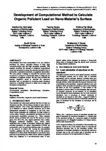
al. (2007). In this modified BC equation, the multiplicative and additive coefficients (e.g. 0.46 and 8) have been recalibrated to cell-specific values (see the resulting coefficient values in Fig. 1). This was done by linearly regressing the cell specific long-term average mean monthly CFSR temperature to the CRU derived long-term average monthly PET for the complete period with overlapping data available for the two datasets (1979–2002). The slopes and intercepts of this linear regression exercise were used to calculate the coefficient values. For the empirical BC equation, which considers only limited meteorological variables, a cell specific recalibration was preferred (this is also illustrated by the large spatial variation in bias between BC PET derived from CFSR data and reference PM PET derived from CRU data, as will be presented in the results section). The HG equation was also applied in its original form (HGorig) and in a re-calibrated form (HGrecal). The HG equation is recognized as an efficient empirical equation with low input data demand, while it integrates consistent information on the spatial variability of climate conditions such as the daily temperature range and a spatial radiation pattern. The spatial radiation pattern is defined as a fixed annual cycle with a daily time-step where values vary with latitude and julian day number (Allen, 1998). Preliminary results indicated that the PET time series derived from the CFSR dataset using the original HG (HGorig) equation gave an overall global underestimation of CRU PET (as will be shown in the results section) with little spatial variability. Therefore, instead of a cell-specific re-calibration, we applied a global uniform modification to the HG equation, by increasing uniformly the multiplication factor in the equation for all grid cells from 0.0023 to 0.0031. Similar increases were proposed by Allen (1993) and Droogers and Allen (2002). To determine the optimal value of the multiplication factor the long term average monthly CFSR HGorig time series were linearly fitted against CRU PET. The multiplication factor was then varied with intervals of 0.0001 until the lowest global average Hydrol. Earth Syst. Sci., 16, 983–1000, 2012

a.

b.

Fig. 1. Cell specific values of the coefficients in the re-calibrated Blaney-Criddle equation. The values in (a) replace the number 0.46 and the values in (b) replace the number 8 in the original BlaneyCriddle equation (ET0 = p(0.46T + 8)).

root mean squared difference (RMSD) value was obtained for the monthly average PET time series. 2.4

Global hydrological modelling

The global water balance was modelled with the GHM PCRGLOBWB. For a detailed description and validation of the model, see Van Beek et al. (2011), Van Beek (2008) and Sperna Weiland et al. (2010). It should of course be noted that the influence of biases in PET on modeled AET, runoff and discharge also depends on the GHM used. Therefore the results of this study can not be generalized to all hydrological models. www.hydrol-earth-syst-sci.net/16/983/2012/

F. C. Sperna Weiland et al.: Calculating global potential evaporation from CFSR re-analysis data Each model cell, with a resolution of 0.5 degrees, consists of two vertical soil layers and one underlying groundwater reservoir. Sub-grid parameterization is used for the schematization of surface water, short and tall vegetation and for calculation of saturated areas for surface runoff as well as interflow. Water enters the cell as rainfall and can be stored as canopy interception or snow. Snow is accumulated when temperature is below 0 ◦ C and melts when temperature is higher. Melt water and throughfall are passed to the surface, where they either infiltrate in the soil or become surface runoff. Exchange of soil water is possible between the soil and groundwater layers in both up- and downward direction, depending on soil moisture status and groundwater storage. Total runoff consists of non-infiltrating melt water, saturation excess surface runoff, interflow and base flow. Time series of reference PET are prescribed to the hydrological model and converted to AET internally. Reference potential evapotranspiration is converted into crop-specific potential evapotranspiration using a crop factor (Allen et al., 1998). PCR-GLOBWB distinguishes two land cover types, short and tall vegetation, given the distinctive differences in plant height, canopy cover and root distributions. The aggregation of different vegetation types into two land cover types is expedient from a computation point of view. However, by basing the parameterization of the different land cover types on the Global Land Cover Characterization (GLCC 2; Loveland et al., 2000) database which has a resolution of 30 arc seconds, much of the sub-grid variability in vegetation conditions can be preserved at the 0.5 degree resolution. Also, although the imposed potential evapotranspiration is called crop-specific, it should be noted that this concerns both natural and cultivated areas. To account for seasonal variations in the crop-specific evaptranspiration, the crop factor is represented by a monthly climatology that reflects the phenology and in case of cultivated surfaces, also the crop calendar. Crop-specific potential evapotranspiration needs to be partitioned into two fluxes, one through the soil matrix (bare soil evaporation) and one through the roots and stomata of vegetation (transpiration). Since vegetation stands are layered and ground cover variable, a break-down on the basis of the minimum crop factor and that of the stand as a whole is preferred over one on the basis of cover fraction. Adopting the upper value for the minimum crop factor (0.2, Allen et al., 1998), the potential evaporation and transpiration flux become: ES0 = ks PET

(1)

T0 = kc PET

(2)

where PET is reference PET (m day−1 ), ks is the “crop factor” used for bare soil, ES0 is potential bare soil evaporation (m day−1 ), kc is the monthly crop factor and T0 is potential crop specific transpiration (m day−1 ). The aggregation of crop types to two vegetation classes on a grid with www.hydrol-earth-syst-sci.net/16/983/2012/

987

a resolution of 0.5 degrees is a simplification of real world vegetation and will in the end impact calculated PET fields. Potential bare soil evaporation and plant transpiration are reduced to AET based on soil moisture conditions. As subgrid variation in soil water storage capacity is considered, part of the surface area may be saturated (Improved Arno Scheme; Hagemann and Gates, 2003). Over this saturated area, potential bare soil evaporation can be sustained as long as the rate does not exceed the saturated hydraulic conductivity. Similarly, over the fraction of the cell where the surface remains unsaturated, the rate is limited by the unsaturated hydraulic conductivity. In the case of transpiration, no transpiration can occur over the saturated part due to oxygen stress, while over the unsaturated area the rate diminishes between full to no transpiration from field capacity to wilting point as a result of water stress. Bare soil evaporation is capable of exhausting soil moisture in the upper soil layer of the model only, whereas transpiration can draw from both layers given the root distribution. For each daily time-step the water balance, and its resulting runoff and AET fluxes, are computed for all model cells. The cell specific runoff is accumulated and routed as river discharge along the drainage network taken from the global Drainage Direction Map (DDM30; D¨oll and Lehner, 2002) using the kinematic wave approximation of the Saint-Venant equation. Due to the coarse resolution of this large scale hydrological model, river discharge can only reliably be calculated for large river basins. 2.5

Statistical validation

The six PET time series derived from CFRS data were validated for the period 1979 to 2002 against monthly CRU based PM PET time series (CRUPM) and compared with each other, using six statistical quantities: 1. A first simple comparison was made by calculating global maps with biases in long-term average annual means: BIAS = PETCFSR − PETCRU

(3)

where PETCFSR refers to annual average PET calculated from the CFSR dataset using one of the six equations (Table 2) and PETCRU refers to the annual average PET calculated from the CRU datasets with the PM equation. Unfortunately, there are no reference global gridded time series of AET available. V¨or¨osmarty et al. (1998) apply an approximation of observed AET by subtracting observed runoff from observed PR. Yet, within their study it is already stated that this approximation is only valid in areas with little water regulation or abstractions and reliable PR and discharge measurements. And, as was also the case for several locations in their study, we obtained negative AET values for a number of basins with this method. Therefore we concluded Hydrol. Earth Syst. Sci., 16, 983–1000, 2012

988

F. C. Sperna Weiland et al.: Calculating global potential evaporation from CFSR re-analysis data (CV) have been calculated from long-term average PET maps calculated with the six different PET equations:

that the method is not reliable when applied to the selected global datasets. As a consequence, the CFSR derived AET and runoff maps are only validated by a comparison between methods.

s

2. To illustrate the significance of the biases calculated in step one, global significance maps have been calculated for PET, AET and local runoff independently. Hereto the significance of the differences between annual average CRU and CFSR derived time series have been quantified with the Welch’s t-test (Welch, 1947) for a significance level of 95 %. The Welch’s adaptation of the standard student’s t-test is used when the two samples possibly have unequal variances. X CRU − XCFSR t= r 2 sCRU nCRU

+

CV =

N

(5)

where PETCFSR refers to the monthly PET calculated from the CFSR data set, PETCRU refers to the monthly PM-based PET calculated from the CRU dataset, i is the month number and N is the total number of months (N = 288). 4. Global maps with long-term annual and seasonal average PET, AET and runoff have been calculated to illustrate the differences between methods while moving through the hydrological model chain. 5. To quantify the variation between the six different equations, cell specific values of the coefficient of variation Hydrol. Earth Syst. Sci., 16, 983–1000, 2012

PETj

M

(6)

6. Performance of the different methods for the reproduction of correct AET amounts is more explicitly evaluated by comparing long-term average modeled river discharge with discharge observations. To this end, annual average discharge is modeled with PCR-GLOBWB forced with temperature, PR and PET from the CFSR dataset for a selection of 19 large rivers (Sperna Weiland et al., 2010). For validation, observed discharge was obtained from the Global Runoff Data Centre (GRDC; GRDC, 2007). The data was adjusted by adding an estimation of water use (Wada et al., 2010; Sperna Weiland et al., 2010).

Where X CRU is the long-term annual average PET, AET or runoff value calculated from the CRU dataset and XCFSR is the long-term annual average calculated from the CFSR dataset for one of the six equations, SCRU is the standard deviation CRU derived annual average PET, AET or runoff values (for all variables 24 annual values over the period 1979 to 2002) and SCFSR is the standard deviation of the 24 CFSR derived annual average values, nCFSR and nCFSR are the number (24) of annual average values for both datasets.

RMSD =

(PETk,j −PETj )2

In addition, global average CV values have been calculated for PET, AET, runoff and discharge and basin specific CV values have been calculated from the annual average river discharge.

(4)

v u N uP u (PETCRUi − PETCFSRi )2 t i=1

j =1

K P k=1

Where PETj is the average of PET calculated with the 6 equations for the specific cell j . PETk,j is the PET calculated for the kth equation for cell j , K is the total number of equations (6), M is the total number of grid cells.

2 sCFSR nCFSR

3. To analyze the seasonal varying character of the biases, global maps with cell specific RMSD (m day−1 ) of the monthly time series (Eq. 5) have been created. These maps give an indication of regional performance on the smallest time-scale at which the validation data is available:

1 K

M P

3 3.1

Results Impact of differences in individual meteorological variables from the CFSR and CRU datasets on PM PET

Global maps with the bias of monthly CFSR-CRU derived PM PET from daily CFSR PM PET are shown for all four seasons in Fig. 2. Within all these maps PET is calculated with the PM equation. Yet, in the top row the daily average CFSR data is replaced by monthly averages in the calculation of PM PET. The maps show that there is limited difference in seasonal averages when using either CFSR daily or CFSR monthly average values as input to the PM equation (Fig. 2a). Therefore, the CFSR PET time-series can be evaluated on a monthly time-scale with CRU data. To evaluate the influence of differences in individual atmospheric variables from the CFSR and CRU dataset, in each row one CFSR variable is replaced with its corresponding CRU variable. Replacing CFSR monthly temperature with CRU monthly temperature does mainly introduce noticable difference over summer in Australia, Central Asia and southen Australia (Fig. 2b). When replacing CFSR radiation with radiation derived from the daily lattitudinal varying www.hydrol-earth-syst-sci.net/16/983/2012/

F. C. Sperna Weiland et al.: Calculating global potential evaporation from CFSR re-analysis data

b.

CFSR monthly DJF

CFSR monthly MAM

CFSR monthly JJA

CFSR monthly SON

CFSR CRU tmp DJF

CFSR CRU tmp MAM

CFSR CRU tmp JJA

CFSR CRU tmp SON

CFSR CRU rad DJF

CFSR CRU rad MAM

CFSR CRU rad JJA

CFSR CRU rad SON

e. CFSR CRU wnd DJF

CFSR CRU wnd MAM

CFSR CRU wnd JJA

CFSR CRU wnd SON

CFSR CRU vap MAM

CFSR CRU vap JJA

CFSR CRU vap SON

c.

d.

f.

CFSR CRU vap DJF

989

Fig. 2. Global maps with bias of monthly CFSR-CRU derived Penman-Monteith potential evaporation (m day−1 ) from daily PenmanMonteith potential evaporation calculated from the daily CFSR time-series for all four seasons. From top to bottom: bias for (b) the full CFSR dataset where al input variables are aggregated to a monthly time-step, (c) the CFSR datasets aggregated to monthly values and temperature replaced with CRU TS2.1 values, (d) the CFSR datasets aggregated to monthly values and incoming radiation derived from an annual sinusoidal radiation cycle and the CRU TS2.1 cloud cover, (e) the CFSR datasets aggregated to monthly values and wind from the CRU CL 1.0 dataset, (f) the CFSR datasets aggregated to monthly values and vapor pressure from the CRU TS2.1 time-series.

radiation cycle reduced with the CRU TS2.1 cloud clover, larger alterations are introduced in the PET fields (Fig. 2c). PET becomes higher over summer in arid regions and lower in humid regions, as for example southern-America and particularly the Amazon. The influence of using a climatological cycle for windspeed is also quite pronounced (Fig. 2d) as could be expexted according to (Roderick et al., 2007). With the CRU climatological wind data PET is overall reduced in the SON and DJF seasons over most of the Southern Hemisphere and in the JJA season over the Northern Hemisphere. Particularly in the MAM and JJA season, PET increases over the Sahara when using climatiological wind fields. Finally, replacing the vapor pressure obtained from the CFSR dataset (which is calculated from an approximiation using the minimum air temperature for the dew-point temperature; Allen et al., 1998; Sperna Weiland et al., 2010) with the CRU TS2.1 vapor pressure fields does not alter the global pattern a lot (Fig. 2e). Yet, locally, in the Sahara and other desert regions in for example Australia and the south-western US, high PET values are reduced.

www.hydrol-earth-syst-sci.net/16/983/2012/

Overall it can be concluded that especially the difference introduced by using climatological radiation and wind instead of their CFSR equivalents is large. Differences introduced by using the CRU temperature are smaller, the difference introduced by using CRU vapor pressure is negligible. 3.2 3.2.1

Evaluation of global potential evaporation Long-term average annual bias

The biases in long-term annual average between CFSR PET and CRU PM PET depend on the PET equation used (Fig. 3). For instance, CFSR PM PET (CFSRPM) underestimates CRUPM in arid regions (e.g. the Sahara, Central Australia and the southwest of the US) and slightly overestimates CRUPM in southeast Asian Islands and parts of the Amazon basin (Fig. 3a). The standard HG equation (CFSRHGorig) underestimates CRUPM globally (Fig. 3b). Yet, a strong correlation between the CFSR HG fields and the CRU PM fields exists. This is amongst others resulting from the fact that both methods use the same latitudinal varying annual Hydrol. Earth Syst. Sci., 16, 983–1000, 2012

990

F. C. Sperna Weiland et al.: Calculating global potential evaporation from CFSR re-analysis data

a) PM

d) PT

b) HGorig

e) HGrecal

c) BCorig

f) BCrecal

Fig. 3. Global maps with annual average bias of CFSR estimated daily reference potential evaporation (PET; m day−1 ) from annual average CRU Penman-Monteith reference PET. In the left column bias in PET obtained with the Penman-Monteith (PM), the standard Hargreaves (HGorig) and Blaney-Criddle (BCorig) method are displayed. In the right column bias obtained with Priestley-Taylor (PT), Hargreaves with increased multiplication factor (HGrecal) and the re-calibrated Blaney-Criddle equation (BCrecal) are displayed.

cycle for radiation. PET calculated with the BC equation (CFSRBC) is too high for almost the entire world (Fig. 3c). Overestimations are especially large in Central Africa and Central South-America. The PT equation (CFSRPT) highly overestimates CRUPM in the Amazon basin, Central Africa and Indonesia, whereas underestimations similar to those of PM CFSR PET are present in the Sahara and parts of Australia (Fig. 3d). By increasing the multiplication factor of the HG equation from 0.0023 to 0.0031, the lowest global average RMSD was obtained (Fig. 3e). PET calculated with the re-calibrated BC equation from the CFSR dataset (CFSRBCrecal) results in highest similarity with CRUPM (Fig. 3f). For illustrational purpose, global maps of absolute PET values are shown for the different methods in the Supplement (Fig. S1). 3.2.2

Comparison of global seasonal PET

Long-term average seasonal PET maps are given in Fig. 4a, b and c. Figure 4a illustrates that CFSR PM PET is overall lower than CRU PM PET (Fig. 4a). Notable differences occur over Australia during the SON and MAM season and Hydrol. Earth Syst. Sci., 16, 983–1000, 2012

over the Sahara throughout the year. Similar deviations over the Sahara can be found for CFSR PT PET, they can be assigned to the radiation fields used to derive CRU PM, as discussed in Sect. 3.2.1. Yet, also in comparison with the HG and BC methods (Fig. 4b and c), PET over the Sahara is low for the PM and PT equations. CRU PM is overestimated by PT PET over the Southern Hemisphere during the DJF season and over the Amazon throughout the year (Fig. 4a). CRU PM is also highly overestimated by the BCorig equation (Fig. 4b). Overestimation is particularly apparent over the Amazon, but also for the summer season in the Northern Hemisphere. The local re-calibration of the BC equation markedly reduces the bias from CRU PM and only small differences can be found, as for example in the MAM and SON season in sub-Arctic regions. However, due to the large spatial variability of the re-calibrated BC coefficient values (Fig. 1), the stability of the equation under changing climate conditions is not guaranteed. In addition, the daily BCrecal PET values span a relatively small range (Fig. 5). The extreme daily values are modest compared to daily PET values derived with the other equations (for brevity, only an example of cumulative distribution functions (CDFs) of daily www.hydrol-earth-syst-sci.net/16/983/2012/

F. C. Sperna Weiland et al.: Calculating global potential evaporation from CFSR re-analysis data

991

Fig. 4a. Global maps with seasonal average daily potential evaporation (m day−1 ). CRU derived with the Penman-Monteith equation (left; = reference for validation), CFSR derived with the Penman-Monteith equation (middle; PM) and CFSR derived with the Priestley-Taylor equation (right; PT). From top to bottom the DJF, MAM, JJA and SON seasons.

PET values are given for the Mackenzie, Amazon, Rhine and Zambezi river basins in Fig. 5). This may be a result of the use of the equation on a daily instead of monthly time-step, for which the equation was originally designed. Although the spatial pattern of PET calculated with the HGorig equation highly resembles CRU PET, PET values are globally too low for this method (Fig. 4c). The globally uniform re-calibration of the HG method notably reduces the differences from CRU PM. In summary, the HGrecal and BCrecal method show the highest agreement with CRU PET. This result is confirmed by the RMSD statistics calculated from monthly time series. Lowest RMSD values are calculated for the BCrecal and HGrecal equations (Fig. 6e and f). Although the PT and PM method also perform satisfactorily well for some regions, they highly underestimate PET over the Sahara and Australia during winter.

www.hydrol-earth-syst-sci.net/16/983/2012/

3.3

3.3.1

Impact of different PET equations on actual evapotranspiration and runoff Long-term average annual evapotranspiration and runoff

For the Amazon and Congo basins and the islands of southeast-Asia absolute AET derived from CFSR PET is higher than AET derived from CRU PET, particularly when calculated with the PT and BCorig equations (Fig. 7a, panel PM AET). AET calculated from both BCorig and BCrecal PET is high in Northern Europe and the Eastern US, especially in the JJA season (Fig. 7a, panel BCrecal AET and 7b, panel BCorig AET). These high values result in slightly lower runoff for these regions than obtained from CRU (Fig. 7a, panel BCrecal runoff). Lowest AET values are derived from HGorig PET (Fig. 7b, panel HGorig AET). Highest similarity between CFSR AET and CRU AET is found for the HGrecal and BCrecal (Fig. 7a, panel HGrecal AET and BCrecal AET). For illustrative purposes global Hydrol. Earth Syst. Sci., 16, 983–1000, 2012

992

F. C. Sperna Weiland et al.: Calculating global potential evaporation from CFSR re-analysis data

Fig. 4b. Global maps with seasonal average daily potential evaporation (m day−1 ). CRU derived with the Penman-Monteith equation (left; = reference for validation), CFSR derived with the re-calibrated Blaney-Criddle equation (middle; BCrecal) and CFSR derived with the original Blaney-Criddle equation (right; BCorig). From top to bottom the DJF, MAM, JJA and SON seasons.

maps of seasonal AET values are given in the Supplement (Fig. S2). Figures 7a, b and 8 show that differences in spatial runoff patterns are almost as small as the differences in AET patterns. This is a result of the fact that the runoff flux is influenced by both AET and PR. Runoff is low for the PT and BCorig method (Fig. 7b, panel PT runoff and BCorig runoff). Although increasing the multiplication factor of the original HG equation to 0.0031 resulted in higher PET values, the difference in runoff derived from the two HG time series is still small (Fig. 7a, panel HGrecal runoff and 7b, panel HGorig runoff). Global seasonal runoff maps are provided for the different PET equations in the Supplement (Fig. S3). 3.3.2

Variation between methods

In Fig. 8 the significance of differences (calculated with the Welch’s t-test for a significance level of 95 %) between annual average PET, AET and local runoff derived from CFSR data (with any of the PET equations) and annual average Hydrol. Earth Syst. Sci., 16, 983–1000, 2012

values of the same variables derived from CRU data is indicated. Within Fig. 8 black areas correspond to regions where annual averages of CFSR and CRU PET derived values do not deviate significantly. Large regions without significant deviations of CFSR PET from CRU PET only occur for the BCcal method. The BCorig and HGorig equations obviously result in the largest areas with significant deviations from CRU PET. While moving from PET to AET to local runoff (QL) the areas with significant deviations of CFSR PET from CRU PET decrease in size as differences between the different PET methods decrease due to limited soil moisture availability and the influence of PR on local runoff and discharge. Globally the variability between the six different PET methods also tends to decrease while moving from PET to AET and runoff, as can be seen from the cell specific CV obtained from the PET values calculated across the six different methods (Fig. 9). For instance, the global cell average CV for PET is 0.42, whereas for AET and runoff the CV values are 0.25 and 0.27 respectively. High CV values for PET and AET are obtained for Northern regions and the www.hydrol-earth-syst-sci.net/16/983/2012/

F. C. Sperna Weiland et al.: Calculating global potential evaporation from CFSR re-analysis data

993

Fig. 4c. Global maps with seasonal average daily potential evaporation (m day−1 ). CRU derived with the Penman-Monteith equation (left; = reference for validation), CFSR derived with the re-calibrated Hargreaves equation (middle; HGrecal) and CFSR derived with the original Blaney-Criddle equation (right; HGorig). From top to bottom the DJF, MAM, JJA and SON seasons.

Himalayas. Yet, CV values for runoff are low in these regions due to the relatively low air temperature, small absolute PET amounts and the large influence of PR. High CV values for PET are also present in the Sahara and central Australia. However, soil moisture is limited in these dry regions and AET amounts are comparably low for the different methods resulting in low CV values.

outlets. The influence of PET methods often decreases while moving within the hydrological model chain from PET to AET to discharge, as water availability becomes limited (V¨or¨osmarty et al., 1998). Basin discharge CV values are found to be lower than CV values for local runoff, due to accumulation of processes along the river network (Sperna Weiland et al., 2012a). CV values of river discharge (Q) range between 0.05 and 0.34 and are on average 0.20.

3.4

Overall, our results suggest that the selection of a PET method is of minor relevance for modeled discharge in part of the investigated basins (Oudin et al., 2005). The smallest variations in discharge between the different PET methods are found in the Monsoon influenced catchments where PR dominates discharge patterns. Highest CV values (0.26– 0.30) are obtained for the Zambezi, Murray and Orange, basins in dry climate where PET has a major impact on resulting discharge. High values are also obtained for the Amazon (0.28) and Congo (0.34). In these tropical basins the high variability between PET methods results in high variability in runoff and discharge as well, due to the humid

3.4.1

Impact of different PET equations on river discharge Variation between PET methods

While being illustrative, the differences in runoff obtained from the six methods are hard to distinguish from the global runoff maps (Fig. S3 in the Supplement). Therefore the variation between methods is quantified with basin specific discharge CV values, calculated from the discharges using the different CFSR PET time series are listed in Table 3 for 19 large rivers at measurement stations close to the catchment www.hydrol-earth-syst-sci.net/16/983/2012/

Hydrol. Earth Syst. Sci., 16, 983–1000, 2012

994

F. C. Sperna Weiland et al.: Calculating global potential evaporation from CFSR re-analysis data

PM PT BCorig BCrecal HGorig HGrecal

Number of days

Fig. 5. CDFs of daily potential evaporation (m day−1 ) for a selection of catchments; MacKenzie, Amazon, Rhine and Zambezi.

Fig. 6. Global maps with cell specific root mean square differences (RMSD) calculated between the CFSR derived monthly PET time series and the monthly PET timeseries derived from the CRU dataset with the Penman-Monteith equation. In the left column from top to bottom; Penman-Monteith (PM), the original Hargreaves method (HGorig) and Blaney-Criddle equation (BCorig) and in the right column; Priestley-Taylor (PT), Hargreaves with increased multiplication factor (HGrecal) and the re-calibrated Blaney-Criddle equation (BCrecal) are displayed.

Hydrol. Earth Syst. Sci., 16, 983–1000, 2012

www.hydrol-earth-syst-sci.net/16/983/2012/

F. C. Sperna Weiland et al.: Calculating global potential evaporation from CFSR re-analysis data

a) PM AET

d) PM runoff

b) HGrecal AET

e) HGrecal runoff

c) BCrecal AET

f) BCrecal runoff

995

Fig. 7a. Global maps with on the left annual average daily actual evapotranspiration (m day−1 ) and on the right annual average daily runoff (m day−1 ). From top to bottom, Penman-Monteith (PM), Hargreaves with increased multiplication factor (HGrecal) and re-calibrated Blaney-Criddle (BCrecal).

Table 3. Catchment specific coefficients of variation (CV) derived from long-term annual average modeled discharge for measurement stations closest to the catchment outlets, obtained with PET time series calculated with the six different potential evaporation equations. Catchment Amazon Brahmaputra Congo Danube Ganges Indus Lena MacKenzie Mekong Mississippi

CV (–) 0.28 0.10 0.34 0.19 0.12 0.05 0.10 0.24 0.16 0.31

Catchment

CV (–)

Murray Niger Orange Parana Rhine Volga Yangtze Yellow Zambezi

0.26 0.18 0.29 0.25 0.17 0.28 0.19 0.17 0.30

climate. Contrary to the results of Oudin et al. (2005) this illustrates that for those basins with high CV values, which are unavoidable part of global scale studies, the selection of a PET equation can influence modeled discharge. Only in www.hydrol-earth-syst-sci.net/16/983/2012/

regions where both the CV of runoff generated by the different PET is high and the absolute runoff amounts are of noteworthy value, the selected PET method is likely to have a large impact on modeled runoff and discharge amounts. See for example the Eastern US, parts of Europe, Russia and the Amazon and Congo basin. The decreasing variability between PET methods throughout the modeling chain mainly occurs in arid regions where AET is limited by soil moisture conditions (e.g. the Sahara, Central Australia and the SouthWestern US) or in the dry seasons. 3.4.2

Deviations from observed GRDC discharge

Discharge calculated from CFSR PR, temperature and the different CFSR PET time series are compared with the observed GRDC discharge (corrected for water use) on an annual base (see Fig. 10). According to this analysis the BCorig equation is the best performing equation, the BCrecal method performs second best and the HGorig method also performs well for some basins. The remaining methods show poor performance.

Hydrol. Earth Syst. Sci., 16, 983–1000, 2012

996

F. C. Sperna Weiland et al.: Calculating global potential evaporation from CFSR re-analysis data

a) PT AET

d) PT runoff

b) HGorig AET

e) HGorig runoff

c) BCorig AET

f) BCorig runoff

Fig. 7b. Global maps with on the left annual average daily actual evapotranspiration (m day−1 ) and on the right annual average daily runoff (m day−1 ). From top to bottom, Priestley-Taylor (PT), the original Hargreaves equation (HGorig) and the original Blaney-Criddle equation (BCorig).

Fig. 8a. Maps showing areas where CFSR derived PET, AET and local runoff (QL) significantly deviates according to the Welch’s t-test for a significance level of 95 % from CRU derived values (in grey) and areas where annual average values do not significantly deviate (in black) for the BCorig, BCrecal and HCorig equations.

Hydrol. Earth Syst. Sci., 16, 983–1000, 2012

www.hydrol-earth-syst-sci.net/16/983/2012/

F. C. Sperna Weiland et al.: Calculating global potential evaporation from CFSR re-analysis data

997

Fig. 8b. Maps showing areas where CFSR derived PET, AET and local runoff (QL) significantly deviates according to the Welch’s t-test for a significance level of 95 % from CRU derived values (in grey) and areas where annual average values do not significantly deviate (in black) for the HGrecal, PM and PT equations.

PET

AET

This is likely a result of this discharge comparison being flawed by measurement errors in amongst others observed discharge (McMillan et al., 2010; Vrugt et al., 2005), biases in PR (Fekete et al., 2004; Biemans et al., 2009) and hydrological model structural errors (Beven, 1996; Vrugt et al., 2005). The most extreme model results are compensating for these biases. This can clearly be seen for the BCorig method, which overall results in the lowest discharge values and therefore performs best for the arid basins (e.g. the Murray, Orange, Zambezi and Niger) where the hydrological model generally overestimates observed discharge (Van Beek, 2008). Because of these biases no clear conclusions can be drawn from the comparison.

4 QL

QC

Fig. 9. Cell specific values of the coefficient of variation (CV; –) calculated from the six different potential evaporation methods for potential evaporation (PET), actual evapotranspiration (AET), local runoff (QL) and discharge (QC).

www.hydrol-earth-syst-sci.net/16/983/2012/

Conclusions

In this study six different methods, to globally derive daily PET time series from CFSR reanalysis data, have been evaluated on (1) their resemblance with monthly PET time series calculated from the CRU datasets with the Penman-Monteith equation and (2) their impact on modeled AET, runoff and river discharge and consequently usability for hydrological impact studies. From the analysis above the following conclusions can be drawn: The selection of a PET method appeared to be of minor importance for river flow modeled with the global hydrological model PCR-GLOBWB in basins where the influence of precipitation on runoff is large and in basins where AET is highly limited by water availability. This is illustrated by the decreasing variability between PET methods while moving Hydrol. Earth Syst. Sci., 16, 983–1000, 2012

998

F. C. Sperna Weiland et al.: Calculating global potential evaporation from CFSR re-analysis data

Fig. 10. Long-term average annual basin discharge (km3 yr−1 ) for 19 large river basins derived with PCRGLOB-WB forced with the CFSR dataset where potential evaporation was calculated using one of the six different PET methods (group of bars on the right for each river). As a reference long-term average corrected observed GRDC basin discharge has been included (black; periods do not completely overlap due to limited data availability).

throughout the hydrological modeling chain (i.e. from PET, AET, runoff to discharge) for these basins. Nevertheless the selected PET method is likely to have a high impact on runoff and discharge amounts for some specific regions (e.g. Amazon, Congo and Mississippi regions). This stresses the necessity to select the most accurate and spatially stable PET method. Overall, the re-calibrated forms of the Blaney-Criddle and Hargreaves equations applied to CFSR data seemed to be best suited to derive daily PET times series. Within this study the Penman-Monteith equation, applied to CFSR data, does not outperform the other methods. It should be noted that this may as well be a result of inaccuracies in individual atmospheric variables in the CRU and CFSR datasets. The sensitivity analysis in Sect. 3.1 illustrated that especially the difference in wind and radiation used for the calculation of CFSR and CRU Penman-Monteith potential evaporation introduces large differences. Due to its high input data requirements and its sensitivity to input data accuracy, the PenmanMonteith method is likely to be less suited for climate change studies. Hydrol. Earth Syst. Sci., 16, 983–1000, 2012

However, we pose two critical remarks against the use of the re-calibrated form of Blaney-Criddle method. First, discharge derived with the re-calibrated Blaney-Criddle method is too low compared to the other methods for most basins. Second, the high spatial variability in the Blaney-Criddle recalibrated coefficient values (Fig. 1) suggests that are sensitive towards future changing climate conditions. We therefore recommend the re-calibrated form of the Hargreaves equation for the derivation of consistent daily PET time series from CFSR reanalysis data for global hydrological studies. Due to its small and spatial uniform bias, the modified Hargreaves method performs satisfactorily in multiple climate zones. In its re-calibrated form the multiplication factor was increased from 0.0023 to 0.0031, which significantly decreased the deviations from CRU PET. Yet, to fully confirm that the re-calibrated Hargreaves method is also stable under changing climate conditions, further investigation with future climate datasets is needed. The results of this study can be of great value for future climate impact assessments. The created PET time series are currently being used to downscale daily PET times-series derived from raw GCM data. These downscaled projections are then used to force the global hydrological model PCRGLOBWB which will result in new consistent hydrological projections at the global scale. The global gridded PETtime-series can be downloaded from http://opendap.deltares. nl/thredds/dodsC/opendap/deltares/FEWS-IPCC. Supplementary material related to this article is available online at: http://www.hydrol-earth-syst-sci.net/16/983/2012/ hess-16-983-2012-supplement.pdf. Acknowledgements. The global discharge time series have been obtained from the Global Runoff Data Centre. The CFSR reanalysis products used in this study are obtained from the Research Data Archive (RDA) which is maintained by the Computational and Information Systems Laboratory (CISL) at the National Center for Atmospheric Research (NCAR). NCAR is sponsored by the National Science Foundation (NSF). The original data are available from the RDA (http://dss.ucar.edu) in dataset number ds093.0. H. H. D¨urr was partly funded by the EU FP6 program “Carbo-North” (contract no. 036993), C. Tisseuil was funded by the Biofresh (contract no. 226874) 7th Framework European project and F. C. Sperna Weiland was funded by the Dutch Research Institute Deltares. Edited by: F. Pappenberger

www.hydrol-earth-syst-sci.net/16/983/2012/

F. C. Sperna Weiland et al.: Calculating global potential evaporation from CFSR re-analysis data References Allen, R. G.: Evaluation of a temperature difference method for computing grass reference evapotranspiration, Report submitted to the Water Resources Development and Man Service, Land and Water Development Division, FAO, Rome, 49 pp., 1993. Allen, R. G., Pereira, L. S., Raes, D., and Smith, M.: Crop evapotranspiration: FAO Irrigation and drainage paper 56, FAO, Rome, Italy, 1998. Arnell, N. W.: The effect of cliamte change on hydrological regimes in Europe: a continental perspective, Global Environ. Chang., 9, 5–23, 1999. Arnell, N. W.: Uncertainty in the relationship between climate forcing and hydrological response in UK catchments, Hydrol. Earth Syst. Sci., 15, 897–912, doi:10.5194/hess-15-897-2011, 2011. Beven, K.: A discussion of distributed hydrological modelling, in: Distributed Hydrological Modelling, Abbott MB, edited by: Refsgaard, J. C., Kluwer Academic; 255–278, 1996. Biemans, H., Hutjes, R. W. A., Kabat, P., Strengers, B., Gerten, D., and Rost, S.: Effects of precipitation uncertainty on discharge calculations for main river basins, J. Hydrometeorol., 10, 1011– 1025, doi:10.1175/2008JHM1067.1, 2009. Blaney, H. F. and Criddle, W. P.: Determining water requirements in irrigated areas from climatological and irrigation data, USDA (SCS) TP-96, 48 pp., 1950. Boorman, H.: Sensitivity analysis of 18 different potential evapotranspiration models to observed climatic change at German climate stations, Climatic Change, 104, 729–753, doi:10.1007/s10584-010-9869-7, 2010. D¨oll, P. and Lehner, B.: Validating of a new global 30-minute drainage direction map, J. Hydrol., 258, 214–231, 2002. Droogers, P. and Allen, R. G.: Estimating reference evapotranspiration under inaccurate data conditions, Irrig. Drain. Syst., 16, 33–45, 2002. Ekstr¨om, M., Jones, P. D., Fowler, H. J., Lenderink, G., Buishand, T. A., and Conway, D.: Regional climate model data used within the SWURVE project – 1: projected changes in seasonal patterns and estimation of PET, Hydrol. Earth Syst. Sci., 11, 1069–1083, doi:10.5194/hess-11-1069-2007, 2007. Elshamy, M. E., Seierstad, I. A., and Sorteberg, A.: Impacts of climate change on Blue Nile flows using bias-corrected GCM scenarios, Hydrol. Earth Syst. Sci., 13, 551–565, doi:10.5194/hess13-551-2009, 2009. Fekete, B. M., V¨or¨osmarty, C. J., Roads, J. O., and Willmott, C. J.: Uncertainties in precipitation and their impacts on runoff estimates, J. Climate, 17, 294–304, 2004. Gavilan, P., Lorite, I. J., Tornero, S., and Berengena, J.: Regional calibration of Hargreaves equation for estimating reference ET in a semiarid environment, Agr. Water Manage., 81, 257–281, doi:10.1016/j.agwat.2005.05.001, 2006. GRDC: Major River Basins of the World/Global Runoff Data Centre, D-56002, Koblenz, Federal Institute of Hydrology (BfG), 2007. Hagemann, S. and D¨umenil Gates, L.: Improving a subgrid runoff parameterization scheme for climate models by the use of high resolution data derived from satellite observations, Clim. Dynam., 21, 349–359, 2003 Hargreaves, G. H. and Samani, Z. A.: Reference crop evapotranspiration from temperature, Appl. Eng. Agric., 1, 96–99, 1985. Hargreaves, G. H., Asce, F., and Allen, R. G.: History and evalu-

www.hydrol-earth-syst-sci.net/16/983/2012/

999

ation of Hargreaves evapotranspiration equation, J. Irrig. Drain. E.-ASCE, 129, 53–63, 2003. Higgins, R. W., Kousky, V. E., Silva, V. B. S., Becker, E., and Xie, P.: Intercomparison of Daily Precipitation Statistics over the United States in Observations and in NCEP Reanalysis Products, J. Climate, 23, 4637–4650, doi:10.1175/2010JCLI3638.1, 2010. IPCC: Climate change 2007: Synthesis report – summary for policy makers, 22 pp., 2007. Jensen, M. E.: Discussion of “irrigation water requirements of lawns”, J. Irr. Drain. Div.-ASCE, 92, 95–100, 1966. Kalnay, E., Kanamitsu, M., Kistler, R., Collins, W., Deaven, D., Gandin, L., Iredell, M., Saha, S., White, G., Woollen, J., Zhu, Y., Leetmaa, A., Reynolds, R., Chelliah, M., Ebisuzaki, W., Higgins, W., Janowiak, J., Mo, K. C., Ropelewski, C., Wang, J., Jenne, R., and Joseph, D.: The NCEP/NCAR 40-year reanalysis project, B. Am. Meteorol. Soc., 77, 437–470, 1996. Kay, A. L. and Davies, V. A.: Calculating potential evaporation from climate model data: A source of uncertainty for hydrological climate change impacts, J. Hydrol., 358, 221–239, doi:10.1016/j.jhydrol.2008.06.005, 2008. Kingston, D. G., Todd, M. C., Taylor, R. G., and Thompson, J. R.: Uncertainty in the estimation of potential evapotranspiration under climate change, Geophys. Res. Lett., 36, L20403, doi:10.1029/2009GL040267, 2009. Loveland, T. R., Reed, B. C., Brown, J. F., Ohlen, D. O., Zhu, J., Yang, L., and Merchant, J. W.: Development of a Global Land Cover Characteristics Database and IGBP DISCover from 1-km AVHRR Data, Int. J. Remote Sens., 21, 1303–1330, 2000. Lu, J., Sun, G., McNulty, S. G., and Amatya, D. M.: A comparison of six potential evapotranspiration methods for regional use in the southeastern united states, J. Am. Water Resour. As., 41, 621– 633, 2005. Mahanama, S. P. P. and Koster, R. D.: AGCM biases in evaporation regime: Impacts on soil moisture memory and land-atmosphere feedback, J. Hydrometeorol., 6, 656–669, doi:10.1175/JHM446.1, 2005. Maurer, E. P., Hidalgo, H. G., Das, T., Dettinger, M. D., and Cayan, D. R.: The utility of daily large-scale climate data in the assessment of climate change impacts on daily streamflow in California, Hydrol. Earth Syst. Sci., 14, 1125–1138, doi:10.5194/hess14-1125-2010, 2010. McMillan, H., Freer, J., Pappenberger, F., Krueger, T., and Clark, M.: Impacts of uncertain river flow data on rainfall-runoff model calibration and discharge predictions, Hydrol. Process., 24, 1270–1284, 2010. Michelangeli, P.-A., Vrac, M., and Loukos, H.: Probabilistic downscaling approaches: application to wind cumulative distribution functions, Geophys. Res. Lett., 36, L11708, doi:10.1029/2009GL038401, 2009. Mitchell, T. D. and Jones, P. D.: An improved method of constructing a database of monthly climate observations and associated high-resolution grids, Int. J. Climatol., 25, 693–712, doi:10.1002/joc.1181, 2005. Monteith, J. L.: Evaporation and environment, Sym. Soc. Exp. Biol., 19, 205–234, 1965. New, M., Hulme, M., and Jones, P.: Representing TwentiethCentury space-time climate variability. Part 1: Development of a 1961–90 mean monthly terrestrial climatology, J. Climate, 12, 829–856, 1999.

Hydrol. Earth Syst. Sci., 16, 983–1000, 2012

1000

F. C. Sperna Weiland et al.: Calculating global potential evaporation from CFSR re-analysis data

New, M., Hulme, M., and Jones, P.: Representing TwentiethCentury Space-Time Climate Variability. Part II: Development of 1901–96 Monthly Grids of Terrestrial Surface Climate, J. Climate, 13, 2217–2238, 2000. Oudin, L., Hervieu, F., Michel, C., Perrin, C., Andr´eassian, V., Anctil, F., and Loumagne, C.: Which potential evapotranspiration input for a lumped rainfall-runoff model? Part 2 – Towards a simple and efficient potential evapotranspiration model for rainfall-runoff modelling, J. Hydrol., 303, 290–306, doi:10.1016/j.jhydrol.2004.08.026, 2005. PCMDI: Program for Climate Model Diagnosis and Intercomparison data portal, available at: https://esg.llnl.gov:8443/index.jsp (last access: 20 March 2012), 2010. Piani, C., Weedon, G. P., Best, M., Gomes, S. M., Viterbo, P., Hagemann, S., and Haerter, J. O.: Statistical bias correction of global simulated daily precipitation and temperature for the application of hydrological models, J. Hydrol., 395, 199–215, doi:10.1016/j.jhydrol.2010.10.024, 2010. Priestley, C. H. B. and Taylor, R. J.: On the assessment of surface heat flux and evaporation using large-scale parameters, Mon. Weather Rev., 100, 81–92, 1972. Roderick, L. M., Rotstayn, L. D., Farquhar, G. D., and Hobbins, M. T.: On the attribution of changing pan evaporation, Geophys. Res. Lett., 34, L17403, doi:10.1029/2007GL031166, 2007. Saha, S., Nadiga, S., Thiaw, C., Wang, J., Wang, W., Zhang, Q., van den Dool, H. M., Pan, H. L., Moorthi, S., Behringer, D., Stokes, D., Pe˜na, M., Lord, S., White, G., Ebisuzaki, W., Peng, P., and Xie, P.: The NCEP Climate Forecast System, J. Climate, 19, 3483–3517, 2006. Saha, S., Moorthi, S., Pan, H.-L., Wu, X., Wang, J., Nadiga, S., Tripp, P., Kistler, R., Woollen, J., Behringer, D., Liu, H., Stokes, D., Grumbine, R., Gayno, G., Wang, J., Hou, Y.-T., Chuang, H.Y., Juang, H.-M. H., Sela, J., Iredell, M., Treadon, R., Kleist, D., van Delst, P., Keyser, D., Derber, J., Ek, M., Meng, J., Wei, H., Yang, R., Lord, S., van den Dool, H., Kumar, A., Wang, W., Long, C., Chelliah, M., Xue, Y., Huang, B., Schemm, J.-K., Ebisuzaki, W., Lin, R., Xie, P., Chen, M., Zhou, S., Higgins, W., Zou, C.-Z., Liu, Q., Chen, Y., Han, Y., Cucurull, L., Reynolds, R. W., Rutledge, G., and Goldberg, M.: The NCEP Climate Forecast System Reanalysis, B. Am. Meteorol. Soc., 91, 1015–1057, 2010. Sperna Weiland, F. C., van Beek, L. P. H., Kwadijk, J. C. J., and Bierkens, M. F. P.: The ability of a GCM-forced hydrological model to reproduce global discharge variability, Hydrol. Earth Syst. Sci., 14, 1595–1621, doi:10.5194/hess-14-15952010, 2010.

Hydrol. Earth Syst. Sci., 16, 983–1000, 2012

Sperna Weiland, F. C., van Beek, L. P. H., Kwadijk, J. C. J., and Bierkens, M. F. P.: On the suitability of GCM runoff fields for river discharge modeling; a case study using model output from HadGEM2 and ECHAM5, J. Hydrometeorol., J. Hydrometeorol., 13, 140–154, doi:10.1175/JHM-D-10-05011.1, 2012a. Sperna Weiland, F. C., van Beek, L. P. H., Kwadijk, J. C. J., and Bierkens, M. F. P.: Global patterns of change in runoff regimes for 2100, Hydrol. Earth Syst. Sci. Discuss., accepted, 2012b. Van Beek, L. P. H.: Forcing PCR-GLOBWB with CRU data, Utrecht University, available at: http://vanbeek.geo.uu.nl/ suppinfo/vanbeek2008.pdf (last access: 24 March 2012), 2008. Van Beek, L. P. H., Wada, Y., and Bierkens, M. F. P.: Global monthly water stress: I. Water balance and water availability, Water Resour. Res., online first: doi:10.1029/2010WR009791, 2011. V¨or¨osmarty, C. J., Federer, C. A., and Schloss, A. L.: Potential evaporation functions compared on U.S. watersheds: Possible implications for global-scale water balance and terrestrial ecosystem modeling, J. Hydrol., 207, 147–169, 1998. Vrugt, J. A., Diks, C. G. H., Gupta, H. V., Bouten, W., and Verstraten, J. M.: Improved treatment of uncertainty in hydrologic modeling: Combining the strengths of global optimization and data assimilation, Water Resour. Res., 41, W01017, doi:10.1029/2004WR003059, 2005. Wada, Y., Van Beek, L. P. H., Van Kempen, C. M., Reckman, J. W. T. M., Vasak, S., and Bierkens, M. F. P.: Global depletion of groundwater resources, Geophys. Res. Lett., 37, L20402, doi:10.1029/2010GL044571, 2010. Weiß, M. and Menzel, L.: A global comparison of four potential evapotranspiration equations and their relevance to stream flow modelling in semi-arid environments, Adv. Geosci., 18, 15–23, 2008, http://www.adv-geosci.net/18/15/2008/. Welch, B. L.: The generalization of “Student’s” problem when several different population variances are involved, Biometrika, 34, 28–35, doi:10.1093/biomet/34.1-2.28, 1947. Wilby, R. L., Wigley, T. M. L., Conway, D., Jones, P. D., Hewitson, B. C., Main, J. and Wilks, D. S.: Statistical downscaling of general circulation model output: A comparison of methods, Water Resour. Res., 34, 2995–3008, 1998.

www.hydrol-earth-syst-sci.net/16/983/2012/