AbstractâRecently the inverted generational distance (IGD) measure has been frequently used for performance evaluation of evolutionary multi-objective ...
Difficulties in Specifying Reference Points to Calculate the Inverted Generational Distance for Many-Objective Optimization Problems Hisao Ishibuchi, Hiroyuki Masuda, Yuki Tanigaki and Yusuke Nojima Department of Computer Science and Intelligent Systems Graduate School of Engineering, Osaka Prefecture University Sakai, Osaka 599-8531, Japan {hisaoi@, hiroyuki.masuda@ci., yuki.tanigaki@ci., nojima@}cs.osakafu-u.ac.jp Abstract—Recently the inverted generational distance (IGD) measure has been frequently used for performance evaluation of evolutionary multi-objective optimization (EMO) algorithms on many-objective problems. When the IGD measure is used to evaluate an obtained solution set of a many-objective problem, we have to specify a set of reference points as an approximation of the Pareto front. The IGD measure is calculated as the average distance from each reference point to the nearest solution in the solution set, which can be viewed as an approximate distance from the Pareto front to the solution set in the objective space. Thus the IGD-based performance evaluation totally depends on the specification of reference points. In this paper, we illustrate difficulties in specifying reference points. First we discuss the number of reference points required to approximate the entire Pareto front of a many-objective problem. Next we show some simple examples where the uniform sampling of reference points on the known Pareto front leads to counter-intuitive results. Then we discuss how to specify reference points when the Pareto front is unknown. In this case, a set of reference points is usually constructed from obtained solutions by EMO algorithms to be evaluated. We show that the selection of EMO algorithms used to construct reference points has a large effect on the evaluated performance of each algorithm. Keywords—Evolutionary multi-objective optimization (EMO), many-objective optimization, inverted generational distance (IGD), performance measures.
I. INTRODUCTION Recently, evolutionary many-objective optimization [1] has become a hot topic in the field of evolutionary multi-objective optimization (EMO [2]-[4]). Difficulties in the handling of many-objective problems can be categorized as follows [5]: (1) Difficulties in the search for Pareto optimal solutions, (2) Difficulties in the approximation of the entire Pareto front, (3) Difficulties in the presentation of obtained solutions, (4) Difficulties in the choice of a single final solution, (5) Difficulties in the evaluation of search algorithms. The first category of difficulties has already been pointed out in many studies (e.g., [6]-[10]). The second category can be viewed as a general characteristic feature of many-objective problems. The third category has been addressed by some studies on solution visualization [11]-[13]. The fourth category The work is partially supported by KAKENHI from JSPS (Grant-in-Aid for Challenging Exploratory Research 26540128).
978-1-4799-4467-5/14/$31.00 ©2014 IEEE
is related to solution visualization and preference incorporation [14]-[17]. The fifth category is related to various issues such as heavy computation load of hypervolume calculation [18]-[20] and difficulties of visual examination of search behavior of EMO algorithms [21]-[23]. The second and third categories of difficulties (i.e., difficulties in approximation and visualization) are also related to difficulties in performance evaluation. In this paper, we discuss difficulties in the use of the inverted generational distance (IGD) measure for performance evaluation of EMO algorithms on many-objective problems. More specifically, we focus our attention on difficulties in appropriately specifying a set of reference points used for the calculation of the IGD measure. It is shown through several examples that performance evaluation using the IGD measure strongly depends on the specification of reference points. This is clear from the definition of IGD: The IGD measure of an obtained solution set is calculated as the average distance from each reference point to the nearest solution in the solution set. This issue has already been pointed out in the literature. For example, Knowles & Corne [24] mentioned that “the score is strongly dependent upon the distribution of points in the reference set” as a negative aspect of the D1R measure [25]. The D1R measure, which was denoted as ID in Zitzler et al. [26], can be viewed as the IGD measure with a different distance definition. The aim of this paper is to clearly demonstrate difficulties in appropriately specifying a set of reference points for IGD-based performance evaluation of EMO algorithms for many-objective problems. This is to encourage a more careful specification of reference points (i.e., a more careful use of the IGD measure), which may lead to a more reliable performance evaluation of EMO algorithms on many-objective problems. This paper is organized as follows. In Section II, we briefly explain the IGD measure. In Section III, we discuss difficulties in sampling reference points from a known Pareto front. We show that a large number of reference points are needed for reliable IGD calculation. However, counter-intuitive results can be obtained even when we use a large number of uniformly sampled reference points for IGD calculation. In Section IV, we discuss the specification of reference points for the case where the Pareto front is unknown. Then we examine a simple modification of the IGD measure for many-objective problems in Section V. Finally we conclude this paper in Section VI.
III. DIFFICULTIES IN THE CASE OF KNOWN PARETO FRONTS
In the EMO community, the hypervolume measure [27] has been dominantly used for performance evaluation of EMO algorithms for many years. However, the inverted generational distance (IGD) has been frequently used for many-objective problems in recent studies [28]-[32] since the computational load for hypervolume calculation exponentially increases with the number of objectives. Let us consider the following maximization problem with k objectives: Maximize f ( x ) ( f1 ( x ), f 2 ( x ), ..., f k ( x )) ,
(1)
subject to x X ,
(2)
where f(x) is the k-dimensional objective vector, fi (x) is the ith objective to be maximized, x is the decision vector, and X is the feasible region. We assume that a solution set A is obtained by an EMO algorithm in the objective space as A = {a1, a2, ..., a|A|}, where aj is a point in the objective space. We also assume that a reference point set Z is also given in the objective space as Z = {z1, z2, ..., z|Z|}, which is an approximation of the Pareto front. Then the IGD measure is calculated for the solution set A using the reference point set Z as follows [31]: IGD(Z, A) =
1 |Z | | A| min d ( zi , a j ) , | Z | i 1 j 1
(3)
where d(zi, aj) is a distance between zi and aj in the objective space. In this paper, we use the Euclidean distance as d(zi , aj). The IGD in (3) is the average distance from each reference point zi to its nearest solution in the solution set A. The IGD measure in (3) was used in 1998 by Czyzak & Jaszkiewicz [25] where the weighted achievement scalarizing function was used as d(zi, aj). This measure in [25] was referred to as the D1R measure in [24] and denoted as ID in [26]. The IGD measure with the Euclidean distance was used in 2003 by Bosman & Thierens [33] and Ishibuchi et al. [34]. However, the name of “inverted generational distance (IGD)” was not used in those studies. The name of IGD was first used in 2004 by Coello & Sierra [35] and Sierra & Coello [36].
When the Pareto front of a multi-objective problem is known, it is advisable to sample reference points uniformly from the entire Pareto front as illustrated in Fig. 1 for a twoobjective problem and Fig. 2 for a three-objective problem. The Pareto front is assumed as being a normalized straight line in Fig. 1 and a normalized triangle in Fig. 2, respectively. The reference points in Fig. 1 and Fig. 2 are generated in the same manner as the uniform weight vector specification in MOEA/D [38] and a cellular EMO algorithm [39]. In those studies, a set of uniformly sampled weight vectors w = (w1, w2, ..., wk) is generated for a k-objective problem as follows: w1 w2 wk 1 ,
(4)
H 1 2 wi 0, , , ..., , i 1, 2, ..., k , H H H
(5)
where H is a pre-specified positive integer. All weight vectors satisfying these relations are generated. In Fig. 1 and Fig. 2, the value of H is specified as 20. The value of H can be viewed as a resolution or granularity of reference points. The number of generated reference points is 21 in Fig. 1 and 231 in Fig. 2. 1.0
Maximize f2(x)
II. INVERTED GENERATIONAL DISTANCE (IGD)
Pareto front Reference point 0.0
1.0
Fig. 1. Uniformly sampled 21 reference points (H = 20).
The main advantages of the IGD measure are twofold. One is its computational efficiency: The IGD measure can be easily calculated even for many-objective problems. The other is its generality: The IGD measure usually shows the overall quality of an obtained solution set A (i.e., its convergence to the Pareto front and its diversity over the Pareto front). Thanks to these nice properties, recently the IGD measure has been frequently used to evaluate the performance of EMO algorithms on manyobjective problems in the literature [28]-[32]. As we can see from its definition in (3), the IGD measure is strongly dependent on the distribution of points in the reference point set Z [24]. However, it is not easy to specify reference points appropriately especially for many-objective problems. In this paper, we illustrate difficulties in specifying reference points in Section III for the case of a known Pareto front and Section IV for the case of an unknown Pareto front using some numerical examples. For theoretical discussions on distancebased performance measures, see Schuetze et al. [37].
Maximize f1(x)
f3(x) 1.0
f2(x) 1.0
f1(x) 1.0 Fig. 2. Uniformly sampled 231 reference points (H = 20).
The number of generated weight vectors by (4) and (5) can be calculated as N = H m 1 C m 1 (i.e., N = C Hm 1m 1 [38]). Intuitively, it seems that a resolution of reference points similar to Fig. 1 and Fig. 2 may be needed to approximate the entire Pareto front (i.e., H = 20). In this case, the number of reference points is calculated for a k-objective problem as follows: 1,771 solutions for k = 4 from H =20, 53,130 solutions for k = 6 from H =20, 888,030 solutions for k = 8 from H =20, 10,015,005 solutions for k = 10 from H = 20. It may be impractical to generate more than ten million reference points for the calculation of the IGD measure for a ten-objective problem. However, the use of coarse resolutions of reference points may lead to counter-intuitive results [5]. Let us assume that we have 11 reference points denoted by closed circles for a two-objective maximization problem in Fig. 3 (i.e., the reference point set Z is generated from H = 10). We also assume that two solution sets A and B are given in Fig. 3, where each open circle in the solution set B is placed at the middle point of adjacent closed circles. Each “x” has the same f1 value as the nearest open circle and the same f2 value as the nearest closed circle. For example, the left most “x” is located at (0.05, 0.9) next to the open circle at (0.05, 0.95) and the closed circle at (0.1, 0.9). In Fig. 3, the solution set A is dominated by the solution set B. However, the IGD measure is calculated for A and B as follows:
two solution sets A and B in Fig. 4 (A: 19 points shown by “x”, B: a single open circle at (0.8, 0.8)). In Fig. 4, the solution set A is dominated by the solution set B (i.e., B is better than A). However, the IGD measure is calculated for A and B as IGD(Z, A) = 0.217 < IGD(Z, B) = 0.426. These results incorrectly suggest that A is better than B (whereas A is dominated by B). In Fig. 4, the increase in the number of uniformly sampled reference points does not change the inequality IGD(Z, A) < IGD(Z, B). One idea is to assign a different weight wi to each reference point zi in (3) as IGD(Z, A) =
1 |Z | | A| min wi d ( zi , a j ) . | Z | i 1 j 1
(6)
By assigning a very large weight only to the knee point (i.e., the closed circle at the right-top corner of the L-shape Pareto front) in Fig. 4, the solution set B can be evaluated as being better than the solution set A using the weighted IGD measure. However, an appropriate specification of weights is not easy. Another idea is to generate more reference points around the knee point as shown in Fig. 5, where the solution set B is evaluated as being better than A by the standard IGD measure with no weights. However, an appropriate specification of a biased distribution of reference points is not easy. 1.0
These results incorrectly suggest that A is better than B (whereas A is dominated by B). If we generate 21 reference points in Fig. 1 from H = 20, the IGD measure is calculated as IGD(Z, A) = 0.053 > IGD(Z, B) = 0.037. These results correctly suggest that B is a better solution set than A. This simple example demonstrates the necessity of high resolution of reference points (i.e., many reference points).
Maximize f2(x)
IGD(Z, A) = 0.056 < IGD(Z, B) = 0.071.
1.0 0.0
Pareto front Reference point Solution in A Solution in B
Maximize f1(x)
1.0
0.0
1.0
Pareto front Reference point Solution in A Solution in B
Maximize f1(x)
1.0
Maximize f2(x)
Maximize f2(x)
Fig. 4. L-shape Pareto front and two solution sets A and B.
Fig. 3. Reference points (H = 10) and two solution sets A and B.
Even when a large number of uniformly sampled reference points are given, the IGD measure can be misleading. Let us assume that uniformly sampled 19 reference points are given on the L-shape Pareto front as shown in Fig. 4. We also assume
0.0
Pareto front Reference point Solution in A Solution in B
Maximize f1(x)
1.0
Fig. 5. Use of reference points with a biased distribution.
typical examples of reference point sets are illustrated in Fig. 7, where Z1 includes concentrated reference points around the center of the Pareto front, reference points in Z2 are welldistributed over the entire Pareto front, and Z3 has reference points around the edges of the Pareto front. Totally different results may be obtained with respect to the performance of EMO algorithms when the IGD measure is used together with a different set of reference points in Fig. 7. For example, the use of reference point set Z1 (closed circles) may favor EMO algorithms with strong convergence property. EMO algorithms with strong diversity improvement mechanisms may be highly evaluated by the IGD measure with the reference point set Z2 (“x”). The IGD measure with the reference point set Z3 (open circles) may give a high evaluation to EMO algorithms with strong optimization ability of each individual objective.
Maximize f2(x)
1.0
Pareto front Reference point Solution in A Solution in B
0.0
Maximize f1(x)
1.0
Another idea is to use the distance from each reference point to the nearest dominated region by an obtained solution set as illustrated in Fig. 6. In this case, the IGD measure may lose its intuitively-understandable meaning: Average distance from the Pareto front to the solution set. This idea can be implemented by calculating the distance d(z, a) from a reference point z = (z1, z2, ..., zk) to a solution a = (a1, a2, ..., ak) in the k-dimensional objective space of the kobjective maximization problem as follows: d ( z, a)
k
2 max{0, ( zh ah )} .
h 1
(7)
When a is dominated by z, d(z, a) is the standard Euclidean distance since zh ah 0 holds for h = 1, 2, ..., k in (7). When a and z are non-dominated with each other, each objective h is used in the distance calculation in (7) only when the reference point z has a better (i.e., larger) objective value zh than ah of the solution a. For a minimization problem, (7) is modified as d ( z, a)
k
max{0, ( ah zh )} ,
h 1
2
(8)
in order to use only those objectives for which the reference point z has a better (i.e., smaller) objective value zh than ah. IV. DIFFICULTIES IN THE CASE OF UNKNOWN PARETO FRONTS
Maximize f2(x)
Fig. 6. Distance from each reference point to the dominated region.
Pareto front Reference point in Z1 Reference point in Z2 Reference point in Z3
Maximize f1(x) Fig. 7. Three typical situations of reference points: Concentration on the center of the Pareto front (Z1), uniform distribution over the entire Pareto front (Z2), and emphasis on the edges of the Pareto front (Z3).
As explained using Fig. 7, the specification of reference points in the IGD measure may have a large effect on the performance evaluation result for each EMO algorithm. When we do not know the true Pareto front, it is almost impossible to appropriately specify reference points. In the following, we examine some frequently-used specification methods. Experiment 1: When the performance of EMO algorithms on a multi-objective test problem is to be compared by the IGD measure, the following procedure is often used:
Except for test problems with special structures, the Pareto front of a multi-objective problem is usually unknown. The unknown Pareto front is often approximated by selecting nondominated solutions among all solutions obtained by different EMO algorithms. Multiple runs of an EMO algorithm with a large population and a large number of generations are also used to obtain a good approximation of the Pareto front. A large number of obtained non-dominated solutions are used as reference points to calculate the IGD measure for a solution set from a single run of an evaluated EMO algorithm.
Step 1: Each EMO algorithm is applied to the test problem several times (100 times in this paper). Step 2: All the obtained solution sets in Step 1 are merged into a single solution set. Then only non-dominated solutions are selected. The selected non-dominated solutions are used as a set of reference points. Step 3: Each solution set obtained in each run of each EMO algorithm is evaluated by the IGD measure using the specified reference points in Step 2.
Since we cannot uniformly sample reference points from the true Pareto front, the constructed set of reference points may have special characteristics or severely biased depending on the EMO algorithms used for reference point search. Three
We examine the performance of the following three EMO algorithms using this procedure for multi-objective 500-item knapsack problems with 2, 4, 6, 8 and 10 objectives (i.e., 2-500, 4-500, 6-500, 8-500 and 10-500 problems in [5]):
(1) Standard NSGA-II. (2) Focused NSGA-II with modified objectives to focus on the center region of the Pareto front. Each objective of the kobjective problem is modified as gi ( x )
1 k f j ( x ) 0.1 f i ( x ) , i = 1, 2, ..., k. k j 1
(9)
(3) MOEA/D with the weighted Tchebycheff. Our computational experiments were performed using the following settings in the same manner as our former study [5]:
However, each table uses a different set of reference points. For example, we show two sets of reference points for the 10500 problem in Fig. 8 using the parallel coordinates. The two sets of reference points in Fig. 8 are also shown in the f1-f2 subspace in Fig. 9. In Fig. 10, we show the projection on the f1f2 subspace of all solutions obtained by 100 runs of each NSGA-II version on the 10-500 problem. Tables I-II and Figs. 8-10 show that the reference solutions with large diversity in Fig. 8 (a) and Fig. 9 (a) favor solution sets with large diversity in Fig. 10 (a) as we explained using Fig. 7. 20500
Objective Value
Coding: Binary string of length 500, Termination condition: 400,000 solution evaluations, Crossover probability: 0.8 (Uniform crossover), Mutation probability: 2/500 (Bit-flip mutation), Population size: 100 (2-500), 120 (4-500), 126 (6-500), 120 (8-500), 220 (10-500), Neighborhood size (MOEA/D): 10 neighbors.
TABLE II.
EMO Algorithm Standard NSGA-II Focused NSGA-II MOEA/D: PBI (0.1)
AVERAGE IGD (EXPERIMENT 1).
2-500 352.3 944.0 61.7
4-500 904.8 1837.4 534.4
6-500 1192.2 1690.5 765.2
8-500 1700.3 1598.0 856.9
10-500 1794.4 1647.7 1057.2
4-500 1026.6 1277.7 340.5
6-500 1453.9 1334.4 516.7
8-500 1974.4 1165.4 658.9
1
2
3 4 5 6 7 (a) Experiment 1.
8
9
10 Objective
1
2
3 4 5 6 7 (b) Experiment 2.
8
9
10 Objective
19000 17500 16000 14500
AVERAGE IGD (EXPERIMENT 2).
2-500 135.8 643.1 101.5
16000
20500
Objective Value
EMO Algorithm Standard NSGA-II Focused NSGA-II MOEA/D: Tchebycheff
17500
14500
Experimental results are summarized in Table I where the average IGD value over 100 runs of each EMO algorithm is shown for each test problem. We used the Euclidean distance for the IGD calculation. Better (smaller) average IGD values are highlighted by bold between the two versions of NSGA-II. TABLE I.
19000
Fig. 8. Two sets of reference points of the 10-500 problem.
10-500 2033.9 1172.3 750.4
Experiment 2: The PBI function with the penalty parameter 0.1 was used instead of the weighted Tchebycheff function in MOEA/D. Experimental results are summarized in Table II. Better (smaller) IGD values are highlighted by bold between the two versions of NSGA-II. Let us compare the two versions of NSGA-II with each other in Table I and Table II. For the 8-500 and 10-500 problems in Table II, much better results were obtained by the focused NSGA-II than the standard NSGA-II. However, differences in the average IGD values on these test problems between the two versions are small in Table I. Moreover, for the 6-500 test problem, much better results were obtained by the standard NSGA-II in Table I whereas better results were obtained by the focused NSGA-II in Table II. It should be noted that the same solution sets are evaluated in Tables I and II with respect to the two versions of NSGA-II. Let us examine why different evaluation results were obtained in Table I and Table II. In these tables, the two versions of NSGA-II were compared by the IGD measure.
f2
f2
20000
20000
19000
19000
18000
18000
17000
17000
16000
16000
15000 15000 16000 17000 18000 19000 20000
(a) Experiment 1.
f1
15000 15000 16000 17000 18000 19000 20000
(b) Experiment 2.
f1
Fig. 9. Projection on the f1-f2 subspace of the two sets of reference points. f2
f2
20000
20000
19000
19000
18000
18000
17000
17000
16000
16000
15000 15000 16000 17000 18000 19000 20000
(a) Standard NSGA-II.
f1
15000 15000 16000 17000 18000 19000 20000
(b) Focused NSGA-II.
f1
Fig. 10. Projection of all solutions obtained by the two versions of NSGA-II.
Experiment 3: In order to generate a wide variety of better reference points than the above-mentioned two experiments, we applied MOEA/D with the weighted Tchebycheff function to each test problem using much more computation load than the examined EMO algorithms in the above experiments. More specifically, MOEA/D with the weighted Tchebycheff function was applied to each test problem under the following setting: Termination condition: 20,000,000 solution evaluations, Population size: 5000 (2-500), 4960 (4-500), 4368 (6-500), 6435 (8-500), 5005 (10-500), Neighborhood size (MOEA/D): 10% of the population size. As reference points, all non-dominated solutions were selected from a merged solution set of all solutions obtained by 100 runs of the two NSGA-II versions in Experiment 1 and the MOEA/D in Experiment 3. The selected reference points for the 10-500 problem are shown in Fig. 11 in the same manner as in Fig. 8 using the parallel coordinates. They are also shown in Fig. 12 in the same manner as in Fig. 9 using the f1-f2 subspace.
19000
Experiment 4: The weighted Tchebycheff function in Experiment 3 is replaced with the PBI function with the penalty parameter value 0.1 in MOEA/D in Experiment 4. Except for this change, Experiment 4 is performed in the same manner as Experiment 3. The selected reference points for the 10-500 problem are shown in Fig. 13 and Fig. 14. From the comparison between Fig. 11 and Fig. 13, we can see that the reference points in Experiment 4 has smaller diversity than those in Experiment 3. We can obtain the same observation from Fig. 12 and Fig. 14. Using the selected reference points, the solution sets obtained by the two versions of NSGA-II in Experiment 1 and Experiment 2 are evaluated. Experimental results are shown in the bottom two rows with “(E4)” in Table III. From these two rows, we can see that the focused NSGA-II is evaluated as being better for the 8-objective and 10-objective test problems in Experiment 4 whereas the standard NSGA-II is evaluated as being better for all test problems in Experiment 3. This observation clearly shows the strong dependency of the IGD-based performance comparison on the reference points. 20500
17500 16000 14500
10 Objective
1 2 3 4 5 6 7 8 9 Fig. 11. Reference points of the 10-500 problem in Experiment 3. f2 20000
Objective Value
Objective Value
20500
and Fig. 12. In this situation, the obtained solution sets with little diversity by the focused NSGA-II (see Fig. 10 (b)) cannot be highly evaluated by the IGD measure.
19000 17500 16000 14500
1 2 3 4 5 6 7 8 9 10 Objective Fig. 13. Reference points of the 10-500 problem in Experiment 4.
19000 18000 17000 16000 15000 15000 16000 17000 18000 19000 20000
f1 Fig. 12. Projection of the reference points in Fig. 11 on the f1-f2 subspace.
From the comparison between Fig. 8 and Fig. 11 (and also between Fig. 9 (a) an Fig. 12), we can see that the reference points in Fig. 11 have more diversity and better (i.e., larger) objective values than those in Fig. 8. Using the reference points in Fig. 11, the solution sets obtained by the two versions of NSGA-II in Experiment 1 and Experiment 2 are evaluated. Their performance evaluation results are shown in Table III, where their results in Tables I and II are also included (as well as the results in Experiment 4 below). In Table III, E1, E2, E3 and E4 show Experiments 1, 2, 3 and 4, respectively. Better results between the two NSGA-II versions are highlighted by bold for each problem in each experiment. From the two rows with “(E3)” in Table III, we can see that the standard NSGA-II is evaluated as being better for all test problems in Experiment 3. This is because the reference points for each test problem have a large diversity as shown in Fig. 11
f2 20000 19000 18000 17000 16000 15000 15000 16000 17000 18000 19000 20000
f1
Fig. 14. Projection of the reference points in Fig. 13 on the f1-f2 subspace. TABLE III.
AVERAGE IGD (EXPERIMENTS 1-4).
EMO Algorithm Standard NSGA-II (E1) Focused NSGA-II (E1) Standard NSGA-II (E2) Focused NSGA-II (E2) Standard NSGA-II (E3) Focused NSGA-II (E3) Standard NSGA-II (E4) Focused NSGA-II (E4)
2-500 352.3 944.0 135.8 643.1 551.0 1221.1 476.7 1138.7
4-500 904.8 1837.4 1026.6 1277.7 1528.6 2352.4 1266.4 1735.4
6-500 1192.2 1690.5 1453.9 1334.4 1743.7 2394.6 1697.7 1850.6
8-500 1700.3 1598.0 1974.4 1165.4 1971.3 2988.5 2138.4 1829.2
10-500 1794.4 1647.7 2033.9 1172.3 2195.8 2521.5 2229.0 1883.4
Experiment 5 and Experiment 6: In Experiment 3 and Experiment 4, MOEA/D spent 50 times larger computation load than NSGA-II. The termination condition of MOEA/D in those experiments was the evaluation of 20 million solutions while NSGA-II was terminated after evaluating 400 thousand solutions. The reference points for each test problem were generated from a merged set of all solutions obtained from MOEA/D and NSGA-II. One may think that the same set of reference points for each test problem can be obtained by using solutions from only MOEA/D (without using solutions from NSGA-II). In order to examine this issue, NSGA-II is not used to generate reference points in the next two experiments. Experiment 5 is the same as Experiment 3 except that the two versions of NSGA-II are not used to generate reference points. Reference points are selected from solutions obtained from 100 runs of MOEA/D with the weighted Tchebycheff function. Experiment 6 is the same as Experiment 4 except that reference points are selected from solutions obtained by only MOEA/D with the PBI function. In Experiment 5 and Experiment 6, we examine whether the following two relations hold between the reference points and each solution set: (i) no reference point is dominated by any solutions in each solution set, (ii) each solution set is dominated by the set of the reference points. For each test problem, we examine whether those relations hold in each of 100 runs of each version of NSGA-II. Experimental results are summarized in Tables IV and V. Table V shows that the dominance relation between the reference point set and the obtained solution set does not hold in many cases. From Table IV, we can see that some reference points are dominated by solutions in the solution sets. This means that solutions from the two versions of NSGA-II have effects on the generation of the reference points in Experiment 3 and Experiment 4. TABLE IV. PERCENTAGE OF RUNS WHERE NO REFERENCE POINT IS DOMINATED BY ANY OF THE OBTAINED SOLUTIONS.
EMO Algorithm Standard NSGA-II (E5) Focused NSGA-II (E5) Standard NSGA-II (E6) Focused NSGA-II (E6)
2-500 42% 100% 100% 100%
4-500 100% 3% 100% 100%
6-500 8-500 10-500 100% 100% 100% 0% 0% 0% 100% 100% 100% 100% 99% 99%
PERCENTAGE OF RUNS WHERE THE SOLUTION SET IS DOMINATED BY THE REFERENCE POINT SET (EXPERIMENT 4).
TABLE V.
EMO Algorithm Standard NSGA-II (E5) Focused NSGA-II (E5) Standard NSGA-II (E6) Focused NSGA-II (E6)
2-500 4-500 6-500 8-500 10-500 33% 60% 1% 0% 0% 100% 0% 0% 0% 0% 99% 100% 100% 100% 100% 100% 93% 0% 0% 0%
V. MODIFIED DISTANCE CALCULATION FOR IGD In Experiment 3, the focused NSGA-II is evaluated as being inferior to the standard NSGA-II for all test problems by the IGD measure (see Table III). One possible reason for the poor evaluation results of the focused NSGA-II in Experiment 3 is that the situation illustrated in Fig. 4 actually happens due to small diversity of the obtained solutions and large diversity
of the reference points. To examine this issue, we recalculate the average IGD value for each EMO algorithm on each test problem using the modified distance calculation method in (7): In the distance calculation between a solution and a reference point, each objective is used only when the reference point has a better objective value than the solution point. Using the modified distance calculation method in (7), the average IGD values in Table III are recalculated. Recalculated results are shown in Table VI. Only the distance calculation method is different between Table III and Table VI. Exactly the same solution sets and the same reference point sets are used in Table III and Table VI. In Table III, IGD-based comparison between the two versions of NSGA-II strongly depends on the specification of the reference point sets. For example, the standard NSGA-II is evaluated as better for all the five test problems in Experiment 3 whereas the focused NSGA-II is evaluated as better for the three test problems in Experiment 2. However, in Table VI, almost the same observations can be obtained from each of the four experiments with respect to the comparison of the two NSGA-II versions. TABLE VI.
AVERAGE IGD WITH THE MODIFIED DISTANCE CALCULATION METHOD IN (7).
EMO Algorithm Standard NSGA-II (E1) Focused NSGA-II (E1) Standard NSGA-II (E2) Focused NSGA-II (E2) Standard NSGA-II (E3) Focused NSGA-II (E3) Standard NSGA-II (E4) Focused NSGA-II (E4)
2-500 179.5 568.6 90.3 435.3 268.3 699.9 264.5 692.3
4-500 702.9 737.1 998.3 810.3 1158.0 1145.6 1169.1 1082.2
6-500 1059.4 580.0 1432.2 823.1 1451.0 1114.8 1635.7 1172.7
8-500 1613.7 518.3 1957.3 573.1 1666.6 1162.9 2103.7 1124.5
10-500 1687.9 502.7 2008.3 539.8 1916.7 1023.4 2187.0 1148.6
VI. CONCLUDING REMARKS In this paper, we clearly demonstrated the following difficulties in the specification of a reference point set for the calculation of the IGD measure. (i) A large number of reference points are needed for reliable performance evaluation of solution sets by the IGD measure. (ii) The number of required reference points exponentially increases with the number of objectives. (iii) Even when a large number of uniformly sampled reference points are given along the entire Pareto front of a twoobjective problem, misleading results can be obtained. (iv) When non-dominated solutions among obtained solutions by examined EMO algorithms are used as reference points, the comparison result depends on the choice of examined EMO algorithms. A change of a setting in a single EMO algorithm can change the IGD-based comparison results among other EMO algorithms. (v) Poor evaluation results are likely to be given to solution sets with good convergence but small diversity especially when reference solutions have large diversity. The use of a modified distance calculation method can remedy such a poor evaluation result on a solution set with small diversity.
REFERENCES [1]
[2] [3] [4] [5]
[6]
[7]
[8]
[9]
[10]
[11]
[12]
[13]
[14]
[15]
[16]
[17]
[18]
[19] [20]
[21]
H. Ishibuchi, N. Tsukamoto, and Y. Nojima, “Evolutionary manyobjective optimization: A short review,” Proc. of 2008 IEEE Congress on Evolutionary Computation, pp. 2424-2431, Hong Kong, China, June 1-6, 2008. K. Deb, Multi-Objective Optimization Using Evolutionary Algorithms, John Wiley & Sons, Chichester, 2001. C. A. C. Coello and G. B. Lamont, Applications of Multi-Objective Evolutionary Algorithms. World Scientific, Singapore, 2004. K. C. Tan, E. F. Khor, and T. H. Lee, Multiobjective Evolutionary Algorithms and Applications. Springer, Berlin, 2005. H. Ishibuchi, N. Akedo, and Y. Nojima, “Behavior of multi-objective evolutionary algorithms on many-objective knapsack problems,” IEEE Transactions on Evolutionary Computation (in press). R. C. Purshouse and P. J. Fleming, “Evolutionary many-objective optimization: An exploratory analysis,” Proc. of 2003 IEEE Congress on Evolutionary Computation, pp. 2066-2073, Canberra, Dec 8-12, 2003. V. Khare, X. Yao, and K. Deb, “Performance scaling of multi-objective evolutionary algorithms,” Lecture Notes in Computer Science 2632: EMO 2003, Springer, Berlin, pp. 376-390, April 2003. E. J. Hughes, “Evolutionary many-objective optimization: Many once or one many?,” Proc. of 2005 IEEE Congress on Evolutionary Computation, pp. 222-227, Edinburgh, September 2-5, 2005. H. Sato, H. E. Aguirre, and K. Tanaka, “Controlling dominance area of solutions and its impact on the performance of MOEAs,” Lecture Notes in Computer Science 4403: EMO 2007, pp. 5-20, Springer, Berlin, March 2007. D. Corne and J. Knowles, “Techniques for highly multiobjective optimization: Some non-dominated points are better than others,” Proc. of 2007 Genetic and Evolutionary Computation Conference, pp. 773780, London, July 7-11, 2007. D. J. Walker, R. M. Everson, and J. E. Fieldsend, “Visualizing mutually nondominating solution sets in many-objective optimization,” IEEE Trans. on Evolutionary Computation, vol. 17, no. 2, pp. 165-184, April 2013. T. Tusar and B. Filipic, “Visualization of Pareto front approximations in evolutionary multiobjective optimization: A critical review and the prosection method,” IEEE Trans. on Evolutionary Computation (in press). F. Kudo and T. Yoshikawa, “Knowledge extraction in multi-objective optimization problem based on visualization of Pareto solutions,” Proc. of 2012 IEEE Congress on Evolutionary Computation, pp. 860-865, Brisbane, Australia, June 10-15, 2012. L. Thiele, K. Miettinen, P. J. Korhonen, and J. Molina, “A preferencebased evolutionary algorithm for multi-objective optimization,” Evolutionary Computation, vol. 17, no. 3, pp. 411-436, Fall 2009. I. Karahan and M. Koeksalan, “A territory defining multiobjective evolutionary algorithms and preference incorporation,” IEEE Trans. on Evolutionary Computation, vol. 14, no. 4, pp. 636-664, August 2010. T. Wagner and H. Trautmann, “Integration of preferences in hypervolume-based multiobjective evolutionary algorithms by means of desirability functions,” IEEE Trans. on Evolutionary Computation, vol. 14, no. 5, pp. 688-701, October 2010. J. H. Kim, J. H. Han, Y. H. Kim, S. H. Choi, and E. S. Kim, “Preference-based solution selection algorithm for evolutionary multiobjective optimization,” IEEE Trans. on Evolutionary Computation, vol. 16, no. 1, pp. 20-34, February 2012. L. While, L. Bradstreet, and L. Barone, “A fast way of calculating exact hypervolumes,” IEEE Trans. on Evolutionary Computation, vol. 16, no. 1, pp. 86-95, February 2012. L. M. S. Russo and A. P. Francisco, “Quick hypervolume,” IEEE Trans. on Evolutionary Computation, vol.18 , no. 4, pp. 481-502, August, 2014. J. Bader and E. Zitzler, “HypE: An algorithm for fast hypervolumebased many-objective optimization,” Evolutionary Computation, vol. 19, no. 1, pp. 45-76, Spring 2011. H. Ishibuchi, Y. Hitotsuyanagi, N. Tsukamoto, and Y. Nojima, “Manyobjective test problems to visually examine the behavior of
[22]
[23]
[24]
[25]
[26]
[27]
[28]
[29]
[30]
[31]
[32]
[33]
[34]
[35]
[36]
[37]
[38]
[39]
multiobjective evolution in a decision space,” Proc. of 11th International Conference on Parallel Problem Solving from Nature, Part II, pp. 91-100, Krakow, Poland, September 11-15, 2010. H. Ishibuchi, N. Akedo, and Y. Nojima, “A many-objective test problem for visually examining diversity maintenance behavior in a decision space,” Proc. of 2011 Genetic and Evolutionary Computation Conference, pp. 649-656, Dublin, Ireland, July 12-16, 2011. H. Ishibuchi, M. Yamane, N. Akedo, and Y. Nojima, “Many-objective and many-variable test problems for visual examination of multiobjective search,” Proc. of 2013 IEEE Congress on Evolutionary Computation, pp. 1491-1498, Cancún, México, June 20-23, 2013. J. D. Knowles and D. W. Corne, “On metrics for comparing nondominated sets,” Proc. of 2002 Congress on Evolutionary Computation, pp. 711-716, Honolulu, May 12-17, 2002. P. Czyzak and A. Jaszkiewicz, “Pareto simulated annealing – A metaheuristic technique for multiple-objective combinatorial optimization,” Journal of Multi-Criteria Decision Analysis, vol. 7, no.1, pp. 34-47, January 1998. E. Zitzler, L. Thiele, M. Laumanns, C. M. Fonseca, and V. G. da Fonseca, “Performance assessment of multiobjective optimizers: An analysis and review,” IEEE Trans. on Evolutionary Computation, vol. 7, no. 2, pp. 117-132, April 2003. E. Zitzler and L. Thiele, “Multiobjective optimization using evolutionary algorithms – A comparative case study,” Lecture Notes in Computer Science, vol. 1498, pp. 292-301, Springer, Berlin, September 1998. S. Yang, M. Li, X. Liu, and J. Zheng, “A grid-based evolutionary algorithm for many-objective optimization,” IEEE Trans. on Evolutionary Computation, vol. 17, no. 5, pp. 721-736, October 2013. Z. He, G. G. Yen, and J. Zhang, “Fuzzy-based Pareto optimality for many-objective evolutionary algorithms,” IEEE Trans. on Evolutionary Computation, vol. 18, no. 2, pp. 269-285, April 2014. M. Li, S. Yang, and X. Liu, “Shift-based density estimation for Paretobased algorithms in many-objective optimization,” IEEE Trans. on Evolutionary Computation, vol. 18, no. 3, pp. 348-365, June 2014. K. Deb and H. Jain, “An evolutionary many-objective optimization algorithm using reference-point based non-dominated sorting approach, Part I: Solving problems with box constraints,” IEEE Trans. on Evolutionary Computation, vol. 18, no. 4, pp. 577-601, August 2014. H. Jain and K. Deb, “An evolutionary many-objective optimization algorithm using reference-point based non-dominated sorting approach, Part II: Handling constraints and extending to an adaptive approach,” IEEE Trans. on Evolutionary Computation, vol. 14, no. 4, pp. 602-622, August 2014. P. A. N. Bosman and D. Thierens, “The balance between proximity and diversity in multiobjective evolutionary algorithms,” IEEE Trans. on Evolutionary Computation, vol. 7, no. 2, pp. 174-188, April 2003. H. Ishibuchi, T. Yoshida, and T. Murata, “Balance between genetic search and local search in memetic algorithms for multiobjective permutation flowshop scheduling,” IEEE Trans. on Evolutionary Computation, vol. 7, no. 2, pp. 204-223, April 2003. C. A. C. Coello and M. R. Sierra, “A study of the parallelization of a coevolutionary multi-objective evolutionary algorithm,” Lecture Notes in Computer Science 2972: MICAI 2004, pp 688-697, April 2004. M. R. Sierra and C. A. C. Coello, A new multi-objective particle swarm optimizer with improved selection and diversity mechanisms, Technical Report of CINVESTAV-IPN, November 23, 2004. (available from http://delta.cs.cinvestav.mx/~ccoello/techreports/evocinv-05-2004.pdf). O. Schuetze, X. Esquivel, A. Lara, and C. A. C. Coello, “Using the averaged Hausdorff distance as a performance measure in evolutionary multiobjective optimization,” IEEE Trans. on Evolutionary Computation, vol. 16, no. 4, pp. 504-522, August 2012. Q. Zhang and H. Li, “MOEA/D: A multiobjective evolutionary algorithm based on decomposition,” IEEE Trans. on Evolutionary Computation, vol. 11, no. 6, pp. 712-731, 2007. T. Murata, H. Ishibuchi, and M. Gen, “Specification of genetic search directions in cellular multi-objective genetic algorithm,” Lecture Notes in Computer Science 1993: EMO 2001, pp. 82-95, Springer, Berlin, March 2001.