Selection Hyper-heuristics in Dynamic Environments - School of ...

Selection Hyper-heuristics in Dynamic Environments Berna Kiraz Institute of Science and Technology, Istanbul Technical University, Turkey

A. “ima Uyar

Department of Computer Engineering, Istanbul Technical University, Turkey

Ender Özcan

School of Computer Science, University of Nottingham, UK

Abstract Current state-of-the-art methodologies are mostly developed for stationary optimization problems. However, many real world problems are dynamic in nature, where dierent types of changes may occur over time. Population based approaches, such as evolutionary algorithms are frequently used in dynamic environments. Selection hyper-heuristics are highly adaptive search methodologies that aim to raise the level of generality by providing solutions to a diverse set of problems having dierent characteristics. In this study, thirty-ve single point search based selection hyper-heuristics are investigated on continuous dynamic environments exhibiting various change dynamics, generated using the Moving Peaks Benchmark generator. Even though there are many successful applications of selection hyper-heuristics to discrete optimization problems, to the best of our knowledge, this study is one of the initial applications of selection hyper-heuristics for real-valued optimization as well as being among the very few which address dynamic optimization issues with these techniques. The empirical results indicate that selection hyper-heuristics with compatible components can react to dierent types of changes in the environment and are capable of tracking them. This shows the suitability of selection hyper-heuristics as solvers in dynamic environments. Keywords: heuristics, meta-heuristics, hyper-heuristics, dynamic environments, moving peaks benchmark, decision support

1 Introduction A hyper-heuristic is a methodology which explores the space of heuristics for solving complex computational problems [8, 40, 13, 11]. Although the term hyper-heuristic is introduced recently [21, 15], the initial ideas can be traced back to the 60s [18, 23]. There has been a growing interest in this eld since then. There are two main types of hyper-heuristics in literature [10]: methodologies 1

that select, or generate heuristics. This study focuses on the former type of hyper-heuristics based on a single point search framework termed as a selection hyper-heuristic.

A selection hyper-

heuristic controls a set of low level heuristics and adaptively chooses the most appropriate heuristic to invoke at each step.

This type of hyper-heuristics have been successfully applied to many

combinatorial optimization problems ranging from timetabling to vehicle routing [9].

In this

paper, from this point on we will use hyper-heuristics to denote selection hyper-heuristics . Real world optimization problems are mostly dynamic in nature. To handle the complexity of dealing with the changes in the environment, an optimization algorithm needs to be adaptive and hence capable of following the change dynamics. From the point of view of an optimization algorithm, the problem environment consists of the instance, the objectives and the constraints. The dynamism may arise due to a change in any of the components of the problem environment. Existing search methodologies have been modied suitably with respect to the change properties to be dealt with in order to tackle dynamic environment problems. A key goal in hyper-heuristic research is raising the level of generality. To this end, approaches which generalize well and are applicable across a wide range of problem domains or dierent problems with dierent characteristics, have been investigated. Considering the adaptive nature of hyper-heuristics, they are expected to respond to the changes in a dynamic environment rapidly and hence be eective solvers in such environments regardless of the change properties. We conducted two preliminary studies on the applicability of hyper-heuristics in dynamic environments in [38, 31]. This study extends our previous work in [31] and further explores the performance of a set of hyper-heuristics in dynamic environments with more realistic change scenarios. Hyper-heuristics have been mostly applied to discrete combinatorial optimization problems in literature [9].

In this study, they are applied to a set of real-valued optimization problems

generated using the Moving Peaks Benchmark (MPB) generator. This benchmark generator is preferred as a testbed for our investigations mainly because it is one of the most commonly used benchmark generators in literature for creating dynamic optimization environments in the continuous domain [19]. The remainder of this paper is organized as follows: next section provides background information on hyper-heuristics and dynamic environments as well as a brief literature survey on the topic; section 3 gives the experimental design and results of the computational experiments, while Section 4 concludes the paper.

2

2 Background 2.1

Selection Hyper-heuristics

In a hyper-heuristic framework, an initial candidate solution is iteratively improved through two

heuristic selection

successive stages:

and

move acceptance

in literature perform a single point based search [9].

[37]. Almost all such hyper-heuristics

In the rst stage, a heuristic is selected

from a xed set of low level perturbative heuristics and applied to the current candidate solution, generating a new one. The heuristic selection method does not use any problem domain specic knowledge while making this decision. Then, the new solution is either accepted or rejected based on an acceptance method. This process is repeated until the termination criteria are satised, after which, the best solution is returned. In the rest of the paper, a hyper-heuristic will be denoted as a

Heuristic Selection Method  Move Acceptance Method

pair.

Cowling et al. [15] dened hyper-heuristics as heuristics to choose heuristics and investigated the performance of dierent heuristic selection methods on a real world scheduling problem. These methods included

Simple Random (SR), Random Descent (RD), Random Permutation (RP), Ran-

dom Permutation Descent method, namely

(RPD),

Choice Function

Greedy

(GR) and a more elaborate learning heuristic selection

(CF). Simple Random selects a low level heuristic randomly.

Random Descent applies a randomly selected heuristic to the current solution repeatedly as long as the solution improves, then another heuristic is selected randomly. Random Permutation randomly orders all low level heuristics and applies each heuristic successively in turns.

Random

Permutation Descent selects a heuristic in the same way as Random Permutation, but it applies the selected heuristic repeatedly as long as the solution improves. Greedy applies all low level heuristics to the current solution and selects the one which generates the largest improvement. Choice Function maintains a utility score for each low level heuristic

Hi

(Equation 1), mea-

suring how well it has performed individually ( u1 (Hi ) in Equation 2) and as a successor of the previously selected heuristic ( u2 (Hi , Hselected ) in Equation 3), and the elapsed time since its last call (u3 (Hi ) in Equation 4). The heuristic with the maximum score is selected at each iteration (Hselected ). The score of each heuristic denoted as selection process. Given that

T imen (y) (T imen (x, y))

Δfn (y) (Δfn (x, y))

score(Hi )

denotes the change in the solution quality and

denotes time spent, when the

3

gets updated after the heuristic

nth

last time heuristic

y

was selected and

applied to the current solution (before the application of heuristic x):

∀i, score(Hi ) ∀i, u1 (Hi ) ∀i, u2 (Hi , Hselected ) ∀i, u3 (Hi )

= αu1 (Hi ) + βu2 (Hi , Hselected ) + δu3 (Hi )  Δfn (Hi ) = αn−1 T imen (Hi ) n  Δfn (Hi , Hselected ) = β n−1 T imen (Hi , Hselected ) n = elapsedT ime(Hi )

(1) (2) (3) (4)

Cowling et al. [16] provide a mechanism showing how the parameters α, β ∈ (0, 1] and δ can be adjusted dynamically. In [15, 17], the authors combined all the above heuristic selection methods with the following move acceptance methods: moves accepted and

All Moves

(AM) accepted,

Improving and Equal (IE) moves accepted.

Only Improving

(OI)

The computational experiments

resulted with the success of the Choice FunctionAll Moves hyper-heuristic. Nareyek [36] applied

Reinforcement Learning (RL) heuristic selection to Orc Quest and mod-

ied logistics domain problems. Reinforcement Learning maintains a utility score (weight) for each low level heuristic. Initially, all scores are the same for all heuristics, e.g., 0. If the selected heuristic improves the solution, its score is increased; otherwise it is decreased, e.g. by one. The scores are restricted to vary between certain lower and upper bounds. The author investigated dierent negative and positive adaptation strategies as well as heuristic selection methods based on the scores.

All Moves

was the acceptance method used in this study. The

results showed that high negative and low positive adaptation rates are preferable. Moreover, the max strategy which selects a heuristic with the maximum score performs better than the softmax (roulette wheel) strategy which chooses a low level heuristic ( Hi ) randomly with a probability of  p(Hi ) = score(Hi )/ ∀j score(Hj ). Apart from the simple acceptance mechanisms, there are other more sophisticated ones. Improving moves are always accepted regardless of the nature of an acceptance mechanism. Kendall and Mohamad [30] applied a

Great Deluge

move acceptance based hyper-heuristic to a mobile

telecommunications network problem. Great Deluge accepts a worsening move, if it is better than a dynamically changing threshold value which depends on the current step and overall duration of the experiment. Linearly decreasing the threshold value at each step is a common practice as illustrated in Equation 5 (for a minimization problem) to determine an acceptance range for a

4

worsening solution. thresholdt = ff inal + ΔF · (1 −

t ) maxIterations

(5)

Here ff inal is the expected nal objective value, maxIterations is the maximum number of steps (or total time), t denotes the current step (time), ΔF is an expected range for the maximum solution quality (tness/cost) change. Ayob and Kendall [1] proposed a set of Monte Carlo move acceptance methods inspired from the well known simulated annealing meta-heuristic. The results showed that Simple Random heuristic selection combined with Exponential Monte Carlo With Counter move acceptance (EMCQ) performs well. EMCQ accepts a worsening move with a probability given in Equation 6, e−

Δf ·m Q

,

(6)

where Q is a counter for successive worsening moves and m is the unit time in minutes that measures the duration of the heuristic execution, Δf is the dierence in the quality between new and current solutions. Q is reset if the quality of the solution improves, otherwise it is incremented. m is incremented at every B steps. Bai et al. [3] showed that Simulated Annealing (SA) as a move acceptance was promising. Bilgin et al. [5] compared the performances of many heuristic selection and move acceptance combinations in hyper-heuristics. The results show that a standard simulated annealing move acceptance performs the best, especially combined with Choice Function. Simulated Annealing accepts all improving moves and a worsening move with a probability given in Equation 7. −

e

ΔF (1−

Δf t ) maxIterations

,

(7)

Bai et al. [2] investigated the performance of a Reinforcement Learning  Simulated Annealing with Reheating (SA+RH) hyper-heuristic on nurse rostering, university course timetabling and one-dimensional bin packing problems. The formula e− is used while deciding whether or not to accept a worsening move. The temperature ( T ) is reduced using the nonlinear formula, T T = 1+γT [34], where Δf T

γ=

(t0 − tf inal )itertemp maxIterations· t0 · tf inal

5

(8)

Here, itertemp is the number of iterations at a temperature. During the reheating phase, the T temperature is increased using the formula T = 1−γT and the system reenters the annealing phase. This hyper-heuristic generates a better performance when compared to the other metaheuristic solutions in each problem domain. The same acceptance was also used by Dowsland et al. [22] as a part of a hyper-heuristic which hybridized Tabu Search with Reinforcement Learning as a heuristic selection method. This hyper-heuristic performed well on a shipper rationalization problem. Burke et al. [12] compared the performance of dierent Monte Carlo move acceptance methods over a set of benchmark examination timetabling problems. EMCQ as a move acceptance method delivered a poor performance as compared to Simulated Annealing based methods. SA+RH turned out to be very promising as a move acceptance component of a hyper-heuristic. Özcan et al. [39] experimented with Great Deluge based hyper-heuristics on examination timetabling. It was observed that Reinforcement LearningGreat Deluge delivers a promising performance, when an additive/subtractive adaptation rate is used for rewarding/punishing. Similarly, Gibbs et al. [24] reported the success of Reinforcement LearningGreat Deluge and Reinforcement Learning Simulated Annealing for solving sports scheduling problems. More on hyper-heuristics can be found in [8, 9, 13, 40]. 2.2

Dynamic Environments

A dynamic environment is made up of components, such as, the problem instance, the objectives and the constraints, each of which may change in time individually or simultaneously. A change in a component can be categorized based on its characteristics as given in [7]: (i) Frequency of change denes how often the environment changes. (ii) Severity of change denes the magnitude of the change in the environment. (iii) Predictability of change is a measure of correlation between changes. (iv) Cycle length/cycle accuracy is a property that denes whether the optima return exactly to previous locations or close to them. When designing an optimization algorithm for dynamic environments, one of the main issues for the algorithm to deal with is tracking the moving optima as closely as possible after a change occurs. Another one is being able to react to a change in the environment quickly and adapting to the new environment as fast as possible. Several strategies have been proposed to be used as a part of existing search methodologies for dynamic environments depending on the change properties. These strategies can be grouped into four main categories [29]: (i) maintain diversity at all times, 6

(ii) increase diversity after a change , (iii) use memory, (iv) work with multiple populations. For the approaches which maintain diversity at all times, e.g., as in the random immigrants approach [25], achieving and preserving the right level of diversity is crucial. These approaches are generally more successful in environments where the changes are severe and the change frequency is relatively high. Approaches, such as hypermutation [14] and variable local search [42] increase diversity by increasing the mutation rate when the environment changes. It has been observed that too much diversity disrupts the search process, while too little may not be sucient to prevent premature convergence. These approaches are more suitable for environments where changes are not too severe. Some approaches make use of memory, as in [33, 20, 45, 43], where the evolutionary algorithm remembers solutions which have been successful in the previous environments. These approaches are particularly more useful if a change occurs periodically and a previous environment is reencountered during the search process at a later stage. There are also other approaches with a good performance in dynamic environments, which make use of multiple populations, such as [7, 41]. In these approaches, the population is divided into subpopulations, where each subpopulation explores a dierent part of the search space. Often, the focus of such an algorithm is tracking several optima simultaneously in dierent regions of the search space.

Further details about

dynamic environments can be found in [7, 19, 35, 44].

2.2.1

The Moving Peaks Benchmark

The Moving Peaks Benchmark (MPB) generator introduced by Branke [6], is used in this study for analyzing and comparing the performance of dierent approaches. MPB is a dynamic benchmark function generator which is not as simplied as most of the toy problems in literature. Moreover, MPB exhibits similar properties to real world problems. The MPB generator provides multidimensional and multimodal landscapes with a variety of dierent peak shapes. In MPB, the most commonly used peak shape is the cone. The height, width and the location of each peak is altered whenever a change in the environment occurs. A dynamic benchmark function generated using MPB with cone shaped peaks is formulated as follows:

F (x, t) =

  d  max {Hi (t) − Wi (t) ∗  (xj − Xij (t))2 }

i=1..m

j=1

7

(9)

where m is the number of peaks, d is the number of dimensions, Xij are the coordinates of the peaks in each dimension, Hi and Wi are the heights and widths of the peaks respectively. For example, assume that the current peak coordinates, height and width values of two peaks in a 2-dimensional landscape at the given time tc are as given in Table 1. The function value of a real-valued vector (candidate solution) located at x = (x1 , x2 ) = (10.0, 3.0) is calculated as follows:  max{50.0 − 0.1 ∗ ((10.0 − 2.0)2 + (3.0 − 2.0)2 ),  70.0 − 0.5 ∗ ((10.0 − 20.0)2 + (3.0 − 20.0)2 )}

F ((10.0, 3.0), tc )

=

F ((10.0, 3.0), tc )

=

max{49.19, 60.14}

F ((10.0, 3.0), tc )

=

60.14

Table 1: Example peak coordinate, height and width values of a 2-dimensional landscape with two peaks Peak i Xi1 (tc ) Xi2 (tc ) Wi (tc ) Hi (tc ) 1 2.0 2.0 0.1 50.0 2 20.0 20.0 0.5 70.0 In some applications, a time-invariant base function B(x) is used as part of the benchmark function. In this case, the new MPB function, denoted as G(x, t) becomes G(x, t) = max{B(x), F (x, t)}. When working with the MPB, rstly, the coordinates, heights and widths of the peaks are initialized. Then, every Δe iterations, the heights and the widths of the peaks are changed by adding a normally distributed random variable, while the location of the peaks are also shifted by a vector v of xed length vlength in a random direction. During the search, the height, width and location of each peak are changed according to the following equations: ρ

∈

(10)

N (μ, σ 2 )

Hi (t)

= Hi (t − 1) + height_severity · ρ

(11)

Wi (t)

= Wi (t − 1) + width_severity · ρ

(12)

 i (t) X

 i (t − 1) + vi (t) = X

(13)

where ρ is a random value drawn from a Gaussian distribution N (μ, σ2 ), where μ and σ2 denote its mean and variance set to 0 and 1, respectively and vi (t) is the shift vector which is the linear combination of the previous shift vector vi (t − 1) and a random vector r normalized to vlength. 8

The height_severity, the width_severity and vlength parameters determine the severity of the change in the heights, widths and locations of the peaks respectively. Δe determines the frequency of changes in the environment. The shift vector at time t is calculated as: vi (t) =

vlength ((1 − φ)r + φ vi (t − 1)) |r + vi (t − 1)|

(14)

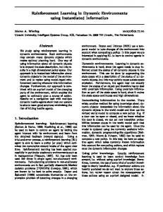
where the random vector r is created by drawing uniformly distributed random numbers for each dimension and normalizing its length to vlength, and φ is the correlation coecient. The higher values of φ indicates a higher correlation between the current and previous shift vectors. Figure 1 gives an example of an initial tness landscape on which various types of changes are applied. The tness landscapes in the gure are generated using MPB with a basis function of B(x) = 0. Figure 1(a) shows the initial 2-dimensional tness landscape with 2 peaks ( m = 2). Each of the rest of the sub-gures shows a specic type of change applied on this initial tness landscape.

=

>

@

?

A

Figure 1: A 2-dimensional tness-landscape with two peaks is given in (a). The following changes are applied on this landscape: (b) the peaks are shifted, i.e. their locations are changed, but their heights and widths remain xed, (c) the widths of the peaks are changed, but their locations and heights remain xed, (d) the heights of the peaks are changed, but their locations and widths remain xed, (e) the heights, widths and locations of the peaks are changed. An initial landscape with ve peaks is generated to demonstrate the eect of the changes on the landscape further. 20 consecutive changes are applied to this initial landscape. For simplicity, only the heights of the peaks are modied as a change, but their locations and widths are xed. 9

Figure 2 gives the height of each peak including the optimum after each change.

70 65 60 peak1 peak2 peak3 peak4 peak5 optimum

Peak Heights

55 50 45 40 35 30 1

2

3

4

5

6

7

8

9 10 11 12 13 14 15 16 17 18 19 20 Environment No

Figure 2: The heights of all the peaks given for each stationary environment over 20 changes.

2.3

Selection Hyper-heuristics in Dynamic Environments

Özcan et al. [38] is the rst study which proposed a hyper-heuristic for solving dynamic environment problems to the best of our knowledge. The authors applied a Greedy hyper-heuristic to ve well known benchmark functions. The Greedy heuristic selection method was chosen as a hyper-heuristic component with the hope that it would respond to the changes in the environment quickly. The results indeed showed that this selection hyper-heuristic is capable of adapting itself to the changes. In [31], the authors compared the performance of dierent heuristic selection mechanisms within the selection hyper-heuristic framework. The hyper-heuristics combined the Improving and Equal acceptance with ve heuristic selection methods controlling a set of mutational low level heuristics in a very simple dynamic environment. The landscape was only allowed to shift in this environment, and its general features remained the same. The Moving Peaks Benchmark was used during the experiments. Choice FunctionImproving and Equal delivered the best average performance. Kiraz and Topcuoglu [32] proposed a population based search framework embedding a variety of hyper-heuristics which combine {Simple Random, Random Descent, Random Permutation, 10

Random Permutation Descent, Choice Function} with {All Moves, Only Improving}. The behavior of these hyper-heuristics is investigated over a set of dynamic generalized assignment problem instances. The authors used an evolutionary algorithm operating on two subpopulations: search and memory. The individuals in the search subpopulation are perturbed using a heuristic selected by a hyper-heuristic and the other one is evolved using a standard evolutionary algorithm updating the memory periodically. The results showed that the Random Permutation DescentAll Moves and Choice FunctionAll Moves hyper-heuristics performed well in general. There is already empirical evidence showing that dierent combinations of hyper-heuristic components yield dierent performances [5, 37] for solving discrete optimization problems. This study extends our previous work in [31] further and provides a complete empirical analysis of dierent hyper-heuristics coupling well known heuristic selection and move acceptance methods in dynamic environments. There is no previous study investigating a single point based search hyper-heuristic framework for solving dynamic environment problems and moreover, to the best of our knowledge, this is one of the rst studies which investigates the application of hyper-heuristics to a real-valued optimization problem.

3 Computational Experiments In this study, we explore the performance of a set of hyper-heuristics in dynamic environments exhibiting dierent change characteristics, which are generated using the MPB generator. The experiments consist of four parts. In the rst part, a simple dynamic environment scenario is investigated, where only the locations of the peaks are changed but their heights and widths remain the same. We will refer to these set of experiments as EXPSET1. In the second part, denoted as EXPSET2, the approaches are compared in environments of dierent change frequencies and change severities, where peak locations as well as peak heights and widths are changed. In the third part, we explore the tracking ability of the approaches. In the last part their scalability is investigated through experiments where the number of peaks and the number of dimensions are increased. 3.1

Experimental Design

We experiment with thirty ve hyper-heuristics composed of ve heuristic selection methods {Simple Random, Greedy, Choice Function, Reinforcement Learning, Random Permutation Descent} 11

combined with seven move acceptance methods {All Moves, Only Improving, Improving and Equal, Exponential Monte Carlo with Counter, Great Deluge, Simulated Annealing, Simulated Annealing with Reheating}. All these hyper-heuristic components have dierent properties. Simple Random uses no feedback. Greedy selects the best solution at each step. Choice Function and Reinforcement Learning incorporate an online learning mechanism. Random Permutation Descent makes a random choice, but converts the framework into a hill climber, since the same heuristic is invoked repetitively as long as the solution improves. Great Deluge, Exponential Monte Carlo with Counter, Simulated Annealing and Simulated Annealing with Reheating are non-deterministic acceptance methods for which the acceptance decision depends on a given step. On the other hand, All Moves, Only Improving, Improving and Equal acceptance methods are deterministic. The hyper-heuristics used in this study are applied to a set of real-valued dynamic function optimization instances produced by the Moving Peaks Benchmark (MPB) generator. A candidate solution is a real-valued vector representing the coordinates of a point in the multidimensional search space for a given instance, for which the length of the vector is the number of dimensions. In order to perturb a given candidate solution, a parameterized Gaussian mutation, N (0, σ 2 ), where σ denotes the standard deviation, is implemented. Seven mutation operators based on seven dierent standard deviations; {0.5, 2, 7, 15, 20, 25, 30} are used as low-level heuristics within the hyper-heuristic framework during the experiments. A low level heuristic draws a random value from the relevant Gaussian distribution for each dimension separately and this random value is added to the corresponding dimension of a candidate solution to generate a new one.

3.1.1

Approaches Used in Comparisons

The performances of dierent hyper-heuristics are compared to well known techniques from literature including a Hypermutation [14] based approach (HM), (1, λ)-Evolutionary Strategies (ES) [4] and (μ,λ)-Covariance Matrix Adaptation Evolution Strategy (CMAES) [26, 28, 27]. These techniques are chosen since they are well known approaches to real-valued optimization and all use a dierent mutation adaptation scheme to deal with the dynamics in the environment. Hypermutation adapts the mutation rate whenever the environment changes. ES adapts the mutation rate based on the success or failure of the ongoing search. In CMAES, adaptation is based on the adaptation of the covariance matrix. The parameter settings of HM, ES and CMAES are determined as a result of a series of preliminary experiments. Hypermutation performs a Gaussian mutation with a xed standard deviation of 2 during

12

the stationary periods. When a change occurs, the standard deviation is increased to

tness evaluations.

consecutive

In (1,λ)-ES,

λ ospring

Afterwards, the standard deviation is reset to

7

σ

is set to

parent

(new candidate solutions) are generated from one

2.

Whenever the environment changes,

During the stationary period of the search, rule [4] as shown in Equation 15 at every denoted as

ps

is greater than

1/5, σ

k

σ

σ

70

2. (current

solution in hand) by a Gaussian mutation with zero mean and a standard deviation of initial value for

for

σ.

The

is reset to this initial value.

is adapted according to the classical

1/5

success

iterations. If the percentage of successful mutations,

is increased, otherwise it is decreased. After

obtained, a solution is selected from them to replace the parent. The value of

k

λ

ospring are

is set to 7. This

evolutionary process repeats until a maximum number of iterations is completed.

⎧ ⎪ ⎪ σ/c ⎪ ⎪ ⎨ σ= σ.c ⎪ ⎪ ⎪ ⎪ ⎩ σ

if

ps > 1/5

if

ps < 1/5

if

ps = 1/5

During the experiments, the value of the parameter

c

(15)

is set to

0.9 ∈ [0.85, 1)

as suggested in [4].

CMAES is the state-of-the-art algorithm for global optimization. It is based on the adaptation

g+1

are generated by sampling the

(g) = xw + σ (g) ∼ N (0, C (g) )

(16)

of the covariance matrix. In CMAES, ospring at generation multivariate normal distribution [28], i.e.

(g+1)

xk where size,

(g)

xw

C (g)

is the weighted mean of the

k = 1, . . . , λ

μ best individuals at generation g , σ

is the covariance matrix at generation

evolution path. The step size

σ

is initialized to

g.

The covariance matrix

σ = 0.3

is the mutation step

C

is adapted via the

and is then updated using a cumulative

step-size adaptation (CSA) approach, in which a conjugate evolution path is constructed [28]. Further details on CMAES can be found in [26, 28, 27]. The initial value of

μ

is set to

1

for CMAES for a fair comparison with the other single point

search methods [28], while the value of

λ for ES and CMAES is set to 7 for a fair comparison with

the Greedy hyper-heuristic which makes

7

evaluations at each step.

13

3.1.2

Parameter Settings of Hyper-heuristics

Some of the heuristic selection and acceptance methods have parameters which require initial settings. • In Reinforcement Learning, the initial scores of all heuristics are set to 15. Their lower and

upper bounds are set to 0 and 30, respectively as suggested in [39]. If the current heuristic produces a better solution than the previous one, its score is increased by 1, otherwise it is decreased by 1. • In Choice Function, α, β , and δ are set to 0.5 and updated by ±0.01 at each iteration. • In Exponential Monte Carlo with Counter, the value of B is set to 60, 10, 2 for LF, MF and

HF changes, respectively. • In Great Deluge, Simulated Annealing and Simulated Annealing with Reheating, the ex-

pected range is calculated as ΔF = initialError −optimumError, where optimumError = 0. Also in Simulated Annealing with Reheating, the starting and nal temperatures are set

to t0 = −ΔF/log(0.1) and tf inal = −ΔF/log(0.005), respectively. It is assumed that all programs are aware of the time when a change occurs during the experiments. As soon as the environment changes, • the current solution is re-evaluated. • the Exponential Monte Carlo with Counter parameters m and Q are reset to 1. • the expected range( ΔF ) is recalculated for Great Deluge and Simulated Annealing. • the system enters the reheating phase for Simulated Annealing with Reheating.

On the other hand, the parameters of the heuristic selection methods Choice Function and Reinforcement Learning are not updated at all when the environment changes.

3.1.3

Experimental Settings

Each run is repeated 100 times for a given setting. Each problem instance contains 20 changes in a given environment, i.e. there are 21 consecutive stationary periods. The total number of iterations per run (maxIterations) is determined based on the change period as given in Equation 17, maxIterations = (N oOf Changes + 1) ∗ ChangeP eriod

14

(17)

where there are (N oOf Changes+1) stationary periods with a length of ChangeP eriod, including the initial environment before the rst change. Table 2 lists the xed parameters of the Moving Peaks Benchmark used during the experiments. These parameter settings are taken from [6, 7]. In the scalability experiments, dimension and peak counts are changed while the rest of the settings are kept the same. Table 2: Parameter settings for the Moving Peaks Benchmark Parameter Setting Parameter Setting Number of peaks p 5 Number of dimensions d 5 Peak heights ∈ [30, 70] Peak widths ∈ [0.8, 7.0] Peak function cone Basis function not used Range in each dimension ∈ [0.0, 100.0] Correlation coecient φ 0 In this study, we experimented with combinations of two change characteristics, namely the frequency and the severity of the changes. We performed some initial experiments to determine the settings for various change frequencies and severities. First, we utilized the Simple Random heuristic selection as a basis to determine change frequency settings. We allowed a Simple RandomImproving and Equal hyper-heuristic to run for long periods without any change in the environment. Based on the resultant convergence behavior, we determined the change periods  as 6006 tness evaluations for low frequency (LF), 1001 for medium frequency (MF) and 126 for high frequency (HF). In the convergence plot, 6006 tness evaluations correspond to a stage where the algorithm has been converged for some time, 1001 corresponds to a time where the approach has not yet fully converged and 126 is very early on in the search. In MPB, the severity of the changes in the locations of the peaks, their heights and widths are controlled by three parameters, namely shift length, height severity and width severity, respectively. We determined low severity (LS), medium severity (MS) and high severity (HS) change settings based on the Moving Peaks Benchmark formulation given in Equation 9. The parameter settings used in the experiments for dierent levels of severity are provided in Table 3. Table 3: MPB parameter settings for each severity level Setting LS MS HS Shift length 1.0 5.0 10.0 Height severity 1.0 5.0 10.0 Width severity 0.1 0.5 1.0  Since we have 7 low level heuristics and the Greedy heuristic selection method evaluates all at each step, these values are determined as multiples of 7 to give each method an equal number of evaluations during each stationary period.

15

3.1.4

Performance Evaluation

The performance of the approaches is compared based on the oine error [7] metric. The error value of a candidate solution x at time t represents its distance to the optimum in terms of the objective/functional value at a given time as given in Equation 18. err(x, t) = |optimum(t) − F (x, t)|

(18)

Here optimum(t) and F (x, t) are the function values of the global optimum solution and a given candidate solution x (see Equation 9) at time t, respectively (MPB provides the location and the function value of the current global optimum). The oine error is calculated as a cumulative average of err(xb , t)∗ which denote the error values of the best candidate solutions ( xb ) found so far since the last change until a given time t, as provided in Equation 20. An algorithm solving a dynamic environment problem aims to achieve the least overall oine error value obtained at the end of a run. 1

T eval

Teval

t=1

(err(xb , t)∗ )

(19)

err(xb , t)∗ = min{err(xb , τ ), err(xb , τ + 1), . . . , err(xb , t)}

(20)

of f line_error =

Here Teval is the total number of evaluations, τ is the last time step (τ < t) when change occurred, and xb is the best solution found so far until the time step t since the last change at time τ . 3.2

Results and Discussion

All trials are repeated for 100 times using each approach for each test case. The results are provided in terms of average oine error values in the tables. The performances of the approaches are compared under a variety of change frequency-severity pair settings where each setting generates a dierent dynamic environment. In the result tables, the best performing approach is marked in bold. The comparisons based on One-way ANOVA and Tukey HSD tests at a 95% condence level are performed to show whether the observed pairwise performance variations are statistically signicant or not. We illustrate the tracking ability of the approaches as well as their scalability, only using EXPSET2 in this section, since we have observed the same behavior for EXPSET1 and EXPSET2. 16

3.2.1

Results for EXPSET1

Table 4 summarizes the results of EXPSET1 using MPB in which only the peak locations change in time. The performance of all methods degrades as the change frequency increases. Moreover, the oine error becomes particularly high when the change frequency is high. Performance also degrades for almost all methods as the severity of change increases. These observations are somewhat expected, based on the fact that the methods are provided with a very limited time to respond to the changes in the environment. We performed statistical signicance tests to determine the overall best heuristic selection and best move acceptance methods. Considering all hyper-heuristic runs where a dierent heuristic selection method is used, Improving and Equal acceptance consistently performs the best over all frequency-severity settings. However, when considering all hyper-heuristic runs where a dierent move acceptance method is used, there is more variation among the best performing heuristic selection methods for dierent frequency-severity settings: •

Greedy performs the best when combined with the All Moves acceptance.

•

Choice Function is the best as a heuristic selection method to be combined with the Improving and Equal, Only Improving and EMCQ acceptance methods.

•

Greedy seems to perform the best for low frequency changes, while the heuristic selection methods that rely on randomness, i.e., RPD and Simple Random perform better for higher frequency changes when combined with Simulated Annealing and Simulated Annealing with Reheating.

•

Great Deluge based hyper-heuristics perform similarly regardless of the heuristic selection.

Overall, considering the average oine error results given in Table 4 and the statistical signicance tests, Choice FunctionImproving and Equal is the best performing hyper-heuristic for EXPSET1. Hypermutation performs the best when combined with the Improving and Equal and Only Improving acceptance methods. However, overall it is one of the heuristic selection methods which delivers very poor performance. Evolutionary Strategies performs well in the cases for which the change frequency is low. Its performance deteriorates as the frequency increases. CMAES performs the best only when both the change frequency and severity are low. For this particular case, ES is the second best performing approach and they are both better than Choice FunctionImproving and Equal. For all the remaining frequency-severity settings, Choice FunctionImproving and Equal performs the best. 17

Table 4: The oine error generated by each approach during the EXPSET1 experiments for dierent combinations of frequency and severity of change. LF Algorithm LS MS GR-AM 24.92 24.69 1.24 2.22 GR-OI GR-IE 1.26 2.23 2.07 4.10 GR-GD GR-EMCQ 2.69 3.67 3.52 7.28 GR-SA GR-SA+RH 6.18 6.74 CF-AM 117.90 117.80 0.64 0.69 CF-OI CF-IE 0.63 0.69 CF-GD CF-EMCQ CF-SA CF-SA+RH SR-AM SR-OI SR-IE SR-GD SR-EMCQ SR-SA SR-SA+RH RL-AM RL-OI RL-IE RL-GD RL-EMCQ RL-SA RL-SA+RH HM-AM HM-OI HM-IE HM-GD HM-EMCQ HM-SA HM-SA+RH RPD-AM RPD-OI RPD-IE RPD-GD RPD-EMCQ RPD-SA RPD-SA+RH ES CMAES

3.2.2

3.18 0.81 6.59 13.11 35.05 0.97 0.97 2.06 1.68 3.70 8.79 38.01 1.39 1.38 2.85 2.59 6.39 11.30 60.44 2.23 2.22 3.74 2.57 5.14 7.83 36.60 0.97 0.96 2.09 1.52 3.56 8.14 0.53

0.42

4.60 0.88 11.45 13.19 34.93 1.19 1.18 4.02 2.08 9.72 8.93 37.73 2.58 2.74 5.92 3.15 12.18 11.46 59.60 2.51 2.50 4.61 2.78 9.14 8.06 36.90 1.13 1.13 3.93 1.80 9.19 8.07

0.65 1.59

HS 24.77 3.38 3.39 5.99 4.76 13.20 8.00 118.10 0.79 0.79 7.16 1.00 19.74 13.92 35.23 1.37 1.38 6.62 2.31 15.96 8.87 37.39 2.97 3.13 9.05 3.46 17.57 11.53 59.58 2.57 2.57 6.11 2.86 14.87 8.45 36.43 1.28 1.28 6.42 1.96 15.04 8.50 0.79 3.15

LS 38.09 3.15 3.06 4.02 4.89 11.47 15.05 155.73 1.25 1.28 3.93 1.51 38.60 26.62 52.96 1.83 1.87 3.33 2.77 6.79 14.45 60.30 2.53 2.73 4.42 5.05 12.52 21.47 88.57 3.47 3.47 5.61 3.92 9.79 14.76 54.86 1.78 1.78 3.24 2.47 6.27 13.83 2.87 1.96

MF MS 37.69 7.42 7.36 8.34 8.20 18.50 16.30 157.35 1.58 1.52

6.27 1.79 42.23 28.88 53.09 2.99 3.01 6.34 4.06 15.02 15.18 61.28 4.32 4.36 10.21 6.13 19.53 21.54 87.00 4.66 4.71 7.36 4.95 15.51 15.33 54.28 2.68 2.68 6.13 3.48 14.16 14.19 3.45 5.60

HS 37.90 12.15 12.18 13.59 12.96 23.71 18.60 155.95 2.17 2.17 10.78 2.46 58.41 28.79 52.76 4.21 4.23 10.29 5.19 24.01 16.04 59.36 5.34 4.86 15.15 6.01 27.69 21.87 87.15 5.23 5.19 9.64 5.50 23.90 14.91 54.40 3.63 3.70 9.87 4.43 23.00 14.96 4.19 10.06

LS 63.92 13.55 13.86 14.73 14.16 38.49 55.97 194.89 4.77 4.49

HF MS 63.04 22.58 22.95 24.19 22.72 43.33 55.86 190.75 7.04 6.69

HS 63.51 31.56 31.52 31.96 31.72 46.48 56.11 182.40 11.45

11.51 8.57 11.74 18.56 4.94 7.15 11.67 140.04 136.46 140.97 66.83 59.19 76.07 86.68 86.45 85.55 5.44 11.29 18.41 5.25 11.47 18.06 6.95 13.07 20.76 6.47 12.13 18.51 40.63 42.20 48.23 31.27 32.62 35.66 96.30 97.23 96.12 7.13 8.64 12.12 6.64 8.84 12.90 8.45 12.01 17.33 7.33 9.47 13.58 47.51 54.81 61.05 38.53 39.57 43.15 113.11 111.65 112.23 8.17 14.50 18.10 8.66 14.60 18.68 9.44 15.81 19.72 9.37 14.76 18.49 56.10 65.38 70.23 31.68 32.93 33.53 88.81 88.96 89.45 5.16 10.41 16.24 5.09 10.27 16.36 6.64 12.24 19.28 6.02 10.73 16.65 39.41 42.66 48.91 30.75 32.66 35.28 11.08 12.67 15.88 9.66 13.57 19.97

Results for EXPSET2

Table 5 summarizes the results of EXPSET2 using MPB in which peak locations, their heights and widths are changed. Similar phenomena as in the previous part are observed during this set of experiments. The methods deteriorate in performance as the change frequency increases. We again performed statistical signicance tests to determine the overall best heuristic selection and best move acceptance methods. Considering all hyper-heuristic experiments for which a dierent 18

move acceptance method is used, the Choice Function heuristic selection outperforms all others, except in the low frequency change cases. Here, RPDEMCQ gives the better average results. In this set of experiments, the Improving and Equal, Only Improving and EMCQ acceptance methods all perform well. In most cases, there is no statistically signicant dierence between them when applied in combination with the Choice Function heuristic selection method. Table 5: The oine error generated by each approach during the EXPSET2 experiments for dierent combinations of frequency and severity of change. Algorithm GR-AM GR-OI GR-IE GR-GD GR-EMCQ GR-SA GR-SA+RH CF-AM CF-OI CF-IE CF-GD CF-EMCQ CF-SA CF-SA+RH SR-AM SR-OI SR-IE SR-GD SR-EMCQ SR-SA SR-SA+RH RL-AM RL-OI RL-IE RL-GD RL-EMCQ RL-SA RL-SA+RH HM-AM HM-OI HM-IE HM-GD HM-EMCQ HM-SA HM-SA+RH RPD-AM RPD-OI RPD-IE RPD-GD RPD-EMCQ RPD-SA RPD-SA+RH ES CMAES

LS 26.47 4.35 4.63 5.11 5.35 5.52 8.88 121.08 3.56 3.66 6.53 4.27 10.30 16.22 37.03 3.89 4.04 5.23 4.78 5.36 10.74 39.62 4.60 4.70 5.80 5.29 8.76 13.91 62.52 5.59 5.44 6.66 5.80 7.50 11.16 38.80 4.26 4.14 5.20 4.28 5.16 10.26 3.69 6.20

LF MS 22.85 8.82 8.96 9.96 8.52 11.10 11.35 98.49 8.97 7.95 11.97 9.09 18.47 20.85 33.09 8.19 7.54 9.63 7.84 12.79 12.97 35.19 9.96 9.02 11.73 8.71 14.86 14.55 56.36 10.63 11.38 11.92 9.90 13.82 14.46 33.99 7.54 8.12 8.87 7.42 12.32 12.30 9.19 13.78

HS 24.86 11.48 11.69 13.09 11.47 17.17 13.81 101.57 11.35 11.57 17.94 12.71 29.43 24.56 35.36 10.24 9.84 12.96 10.23 19.78 14.06 37.29 12.02 12.48 15.76 10.81 21.26 17.27 59.70 13.01 13.48 15.94 12.49 22.14 16.58 36.77 10.17 10.28 14.15 9.34 19.30 13.78 12.74 17.01

LS 39.36 6.19 6.33 7.05 8.35 15.88 16.93 153.90 4.79 4.38 6.83 4.69 37.01 26.89 54.60 5.46 4.96 6.39 5.79 9.06 17.19 63.15 5.94 5.73 7.57 8.00 16.27 24.14 90.72 6.88 6.72 8.91 7.09 12.10 17.69 56.75 5.01 5.00 6.71 5.80 8.51 16.50 6.18 7.86

MF MS 32.98 14.06 15.03 15.04 13.37 20.19 19.29 125.84 10.30 10.46 14.37 9.61 62.23 38.02 47.71 9.65 10.76 13.25 10.04 18.05 19.58 54.41 12.65 12.74 16.37 12.64 22.86 25.01 78.52 13.51 13.09 15.82 12.95 20.13 22.23 48.90 10.19 9.67 12.44 10.01 17.44 19.09 12.21 17.25

HS 35.00 19.14 19.38 20.34 19.50 25.86 22.84 128.53 12.86 12.37 21.64 13.75 78.52 43.50 50.13 13.27 13.60 17.59 14.04 27.41 21.70 56.65 16.01 14.17 22.29 15.94 33.97 27.95 82.27 15.73 15.82 19.79 15.48 32.12 24.34 51.39 12.61 12.54 17.27 13.89 26.67 21.29 15.68 21.28

LS 63.41 17.08 17.06 18.70 17.60 43.31 56.71 185.61 7.46 7.47 11.55 8.60 140.89 69.58 88.27 8.83 8.87 9.87 10.03 44.63 35.85 96.70 9.99 9.35 11.30 10.66 54.44 41.55 115.32 11.41 11.27 12.46 12.59 62.87 35.04 90.22 8.12 8.31 10.12 8.99 42.81 33.40 14.58 15.53

HF MS 52.63 28.16 27.61 27.81 28.80 40.30 47.78 143.96 15.65 14.79 19.86 14.76 119.09 75.29 75.67 18.65 18.46 20.10 18.83 41.90 35.60 82.18 16.67 17.54 20.18 16.94 57.35 44.42 98.13 22.21 23.53 23.95 22.39 72.03 38.31 76.93 17.73 16.65 18.98 17.51 42.63 34.82 21.37 24.17

HS 56.06 36.08 35.59 36.31 36.47 45.14 50.02 146.98 23.24 23.83 29.82 24.78 125.79 85.38 78.21 26.90 27.24 29.26 28.16 50.21 39.64 85.15 25.55 25.33 28.55 25.64 66.82 49.78 101.77 29.32 29.63 30.43 29.49 81.57 42.72 80.70 25.56 26.20 28.36 26.59 51.06 39.29 27.40 31.73

Hypermutation is again among the worst performing heuristic selection methods. Unlike in the 19

previous experiments, in EXPSET2, both ES and CMAES do not perform the best in any of the frequency-severity settings. ES is better than CF-EMCQ only when both the change frequency and severity are low. In other cases, ES and CMAES are outperformed by the Choice Function heuristic selection in combination with either Improving and Equal, Only Improving or EMCQ acceptance methods.

3.2.3

Dynamic Environment Heuristic Search Challenge

Recently, CHESC  Cross-domain Heuristic Search Challenge , a competition on hyper-heuristics was held, which used HyFlex, a tool implemented for research and rapid development of hyperheuristics. In this competition, dierent hyper-heuristics competed for solving problem instances from six dierent problem domains. As a comparison and ranking method, the organisers adopted the Formula 1 scoring system. The top eight approaches are given a score of 10, 8, 6, 5, 4, 3, 2 and 1 points for each problem instance from the best to the worst, successively. The rest of the approaches receive a score of 0. The comparison and the ranking of the approaches are based on the median result generated by each approach over a given number of runs for an instance. The sum of scores over all problem instances determine the nal ranking of an approach. In order to evaluate the performance of hyper-heuristics across dierent dynamic environments and see their relative performance as compared to the state-of-the-art techniques, all approaches are scored in the same way as in CHESC. Considering both EXPSET1 and EXPSET2 with all change frequency-severity combinations, there are 18 dierent problems. Therefore, 180 is the maximum overall score an approach can get. The results are summarized in Table 6, where the overall scores of the best ve approaches are included. As can be seen from the results, Choice FunctionImproving and Equal is the clear winner. Figure 3 shows the histogram of scores for this hyper-heuristic which ranks the rst, second and third among all approaches in a total of sixteen out of eighteen cases. Only when a high severity change occurs at a low frequency, Choice FunctionImproving and Equal performs worse than some others. The top three hyperheuristics use Choice Function as the heuristic selection component. All hyper-heuristics using All Moves, Great Deluge, Simulated Annealing or Simulated Annealing with Reheating as an acceptance component perform poorly with an overall score of 0 regardless of the heuristic selection component. ES ranks eighth with a score of 37, CMAES ranks thirteenth with a score of 11, while all the Hypermutation based methods receive a score of 0 in all cases. http://www.asap.cs.nott.ac.uk/external/chesc2011/

20

Table 6: The overall scores for the top ve approaches. Approach Overall Score Choice FunctionImproving and Equal 136 Choice FunctionOnly Improving 119 86 Choice FunctionEMCQ 72 Random Permutation DescentOnly Improving Random Permutation DescentImproving and Equal 71 7

Number of Occurences

6

5

4

3

2

1

0

10

8

6

5

4

Score

3

2

1

0

Figure 3: Histogram of scores for CFIE over 18 dynamic environment cases. 3.2.4

Tracking Ability of the Approaches

The error values of the best candidate solutions calculated using Equation 18 versus the number of evaluations based on dierent change frequency and severity combinations are plotted in Figure 4 for Choice FunctionImproving and Equal, HypermutationAll Moves, ES and CMAES to illustrate and compare their tracking ability when the environment changes. Choice Function Improving and Equal is chosen as the best performing hyper-heuristic, while HypermutationAll Moves is chosen as a poor approach. ES and CMAES are included as they are known to be among the best real-valued optimization approaches. Figure 6 shows the boxplots for the nal oine error values of the corresponding approaches. In the boxplot, the minimum and maximum values obtained (excluding the outliers), the lower and upper quartiles and the median are shown. The outlier points are also marked. To be able to demonstrate the tracking behavior of the approaches more clearly, we isolated the plots for a medium frequency and a medium severity change scenario from Figure 4, and plotted them in Figure 5. From Figures 4 and 5, it can be observed that when the environment changes, the error values of the best candidate solutions produced by Choice FunctionImproving and Equal, ES and CMAES increase much less than that of HypermutationAll Moves. Moreover, these approaches are able to recover much more quickly, following the optimum. This indicates that Choice FunctionImproving and Equal, ES and CMAES display a good tracking behavior. However, the tracking behavior of HypermutationAll Moves is poor. Choice Function-Improving 21

and Equal performs signicantly better than the Hypermutation-All Moves, ES and CMAES on average during most of the environment changes as illustrated in Figure 6. The average performance of an approach reects upon its tracking behaviour as well. 200

200 CF−IE HM−AM ES CMAES

180

120 100 80 60

140 120 100 80 60

40

40

20

20

0

2

4

6

8

10

Fitness Evaluations

0

12

160

Error of the Best Solution

140

CF−IE HM−AM ES CMAES

180

160

Error of the Best Solution

Error of the Best Solution

160

0

200 CF−IE HM−AM ES CMAES

180

140 120 100 80 60 40 20

0

2

4

4

x 10

6

8

10

Fitness Evaluations

0

12

0

2

4

4

x 10

6

8

10

Fitness Evaluations

12 4

x 10

(a) LF (-LS, MS and HS) 200

200 CF−IE HM−AM ES CMAES

180

120 100 80 60

140 120 100 80 60

40

40

20

20

0

0.2

0.4

0.6

0.8

1

1.2

Fitness Evaluations

1.4

1.6

1.8

0

2

160

Error of the Best Solution

140

CF−IE HM−AM ES CMAES

180

160

Error of the Best Solution

Error of the Best Solution

160

0

200 CF−IE HM−AM ES CMAES

180

140 120 100 80 60 40 20

0

0.2

0.4

4

x 10

0.6

0.8

1

1.2

Fitness Evaluations

1.4

1.6

1.8

0

2

0

0.2

0.4

4

x 10

0.6

0.8

1

1.2

Fitness Evaluations

1.4

1.6

1.8

2 4

x 10

(b) MF (-LS, MS and HS) 200

200 CF−IE HM−AM ES CMAES

180

120 100 80 60

140 120 100 80 60

40

40

20

20

0

500

1000

1500

Fitness Evaluations

2000

2500

160

Error of the Best Solution

140

0

CF−IE HM−AM ES CMAES

180

160

Error of the Best Solution

Error of the Best Solution

160

0

200 CF−IE HM−AM ES CMAES

180

140 120 100 80 60 40 20

0

500

1000

1500

Fitness Evaluations

2000

2500

0

0

500

1000

1500

Fitness Evaluations

2000

2500

(c) HF (-LS, MS and HS)

Figure 4: Comparison of approaches (CF-IE, HM-AM, ES, and CMAES) for the combinations of (a) Low, (b) Medium, (c) High frequencies and severities of change based on the error values of the best candidate solution versus evaluation counts for EXPSET2.

3.2.5

Scalability Results

In this part, we investigate the scalability of the approaches for dierent frequency-severity settings. We performed experiments with dierent number of peaks and dimensions. Table 7 summarizes the results for analyzing the eect of the number of dimensions on performance using EXPSET2 for dierent change frequency and severity combinations. In these experiments, only the best hyper-heuristics {Choice FunctionImproving and Equal, Choice FunctionEMCQ} are considered 22

200

200 HF−LS HF−MS HF−HS

180

160

Error of the Best Solution

Error of the Best Solution

160 140 120 100 80 60

140 120 100 80 60

40

40

20

20

0

HF−LS HF−MS HF−HS

180

0

0.2

0.4

0.6

0.8

1

1.2

Fitness Evaluations

1.4

1.6

1.8

0

2

0

0.2

0.4

0.6

4

x 10

0.8

1

1.2

Fitness Evaluations

1.4

1.6

1.8

2 4

x 10

160

160

140

140

140

120

120

120

100

80

Offline Error

160

Offline Error

Offline Error

Figure 5: A sample plot of the error values of the best candidate solution versus evaluation counts based on medium change frequency and medium severity combination for EXPSET2. The left and right plots show the results for Choice FunctionImproving and Equal and Hypermutation All Moves, respectively.

100

80

100

80

60

60

60

40

40

40

20

20

0

CF−IE

HM−AM

ES

0

CMAES

20

CF−IE

HM−AM

ES

0

CMAES

CF−IE

HM−AM

ES

CMAES

CF−IE

HM−AM

ES

CMAES

CF−IE

HM−AM

ES

CMAES

160

160

140

140

140

120

120

120

100

80

Offline Error

160

Offline Error

Offline Error

(a) LF (-LS, MS and HS)

100

80

100

80

60

60

60

40

40

40

20

20

0

CF−IE

HM−AM

ES

0

CMAES

20

CF−IE

HM−AM

ES

0

CMAES

160

160

140

140

140

120

120

120

100

80

Offline Error

160

Offline Error

Offline Error

(b) MF (-LS, MS and HS)

100

80

100

80

60

60

60

40

40

40

20

20

0

CF−IE

HM−AM

ES

CMAES

0

20

CF−IE

HM−AM

ES

CMAES

0

(c) HF (-LS, MS and HS)

Figure 6: Box-plots of oine error values for a statistical comparison of the approaches (CF-IE, HM-AM, ES, and CMAES) for the combinations of (a) Low, (b) Medium, (c) High frequencies and severities of change using EXPSET2.

23

along with HypermutationImproving and Equal, HypermutationEMCQ, ES and CMAES. As expected, the performance of the hyper-heuristics and ES worsens as the number of dimensions increases. ES seems to be less aected from the dimensionality increase for lower frequency and severity settings. CMAES improves its performance when the number of dimensions is increased to 10. However, Choice FunctionImproving and Equal scales better and is the best performing approach for higher change frequency and severity settings. Table 7: Oine error generated by each approach in the experiments for analyzing the eect of number of dimensions for EXPSET2 for dierent frequency and severity combinations

LS LF MS HS LS MF MS HS LS HF MS HS

# of dimensions 5 10 20 5 10 20 5 10 20 5 10 20 5 10 20 5 10 20 5 10 20 5 10 20 5 10 20

CF-IE CF-EMCQ HM-IE HM-EMCQ ES 3.78 4.52 5.39 5.74 4.14 4.85 5.61 9.22 11.03 4.60 8.22 10.34 17.76 24.09 5.65 9.04 9.29 12.40 10.06 9.73 11.35 11.47 15.91 15.03 9.88 15.46 16.37 26.22 25.76 13.73 10.53 12.02 12.42 12.43 12.16 13.29 15.06 19.99 17.68 12.67 18.21 21.27 32.57 29.62 16.56 4.61 4.79 6.66 7.20 6.35 6.99 7.69 11.33 13.92 9.22 13.34 15.45 21.99 28.51 17.66 10.91 10.23 13.11 13.07 13.10 13.21 14.00 19.89 21.26 17.68 21.00 22.14 33.63 36.96 30.54 13.43 14.06 15.69 15.11 15.67 17.26 18.67 25.47 24.78 23.07 24.94 27.32 41.16 44.28 37.12 8.48 8.50 11.68 13.03 14.04 17.38 19.60 23.22 26.32 31.88 49.53 52.28 48.42 53.73 68.98 15.82 15.56 22.62 23.33 21.26 27.40 28.88 36.73 36.70 40.03 61.30 61.68 64.35 63.72 78.68 24.07 24.39 29.81 29.55 28.32 37.32 38.96 50.78 49.52 46.62 75.16 76.25 78.59 75.79 85.02

CMAES 5.98 2.30 4.75

12.05

7.08 11.94

12.48 14.15 21.84 7.94

5.35 12.46

17.94 22.83 24.23 21.80 33.39 14.70 27.20 73.81 23.18 34.87 86.49 42.36 50.22 86.55

12.31

Table 8 provides the results for analyzing the eect of the number of peaks in the environment on performance using EXPSET2 for dierent change frequency and severity combinations. The same hyper-heuristics {Choice FunctionImproving and Equal, Choice FunctionEMCQ, HypermutationImproving and Equal, HypermutationEMCQ}, ES and CMAES are included in the experiments. Again, the performance of the hyper-heuristics worsens as the number of dimensions increases. This time, ES performs similar to the hyper-heuristics. However, the eect of the increase in the number of peaks is less than the eect of the increase in dimensionality for ES. CMAES improves its performance as the number of peaks increases for all frequencies combined with low and medium severities. However, in almost all cases, it is no longer the best performing 24

approach. All methods seem to scale well with respect to the increase in the number of peaks in the environment. Table 8: Oine error generated by each approach in the experiments for analyzing the eect of number of peaks for EXPSET2 for dierent frequency and severity combinations

LS LF MS HS LS MF MS HS LS HF MS HS

# of peaks 5 10 15 5 10 15 5 10 15 5 10 15 5 10 15 5 10 15 5 10 15 5 10 15 5 10 15

CF-IE CF-EMCQ HM-IE HM-EMCQ ES 3.76 4.00 5.40 5.79 3.95 4.75 4.82 6.27 6.32 4.65 4.83 5.33 6.95 6.83 4.87 9.67 9.05 9.90 10.16 9.07 11.04 11.06 12.72 10.53 10.95 11.47 11.15 12.26 9.73 11.36 11.55 11.27 13.56 12.41 11.33 13.74 14.16 14.55 13.22 14.34 14.52 13.51 15.08 12.28 13.72 4.58 4.43 6.48 7.17 6.23 4.93 5.22 7.36 7.95 6.82 5.87 5.67 7.41 8.33 7.60 9.63 10.42 12.31 11.14 11.46 11.06 12.23 14.45 12.57 13.62 12.41 11.59 14.31 12.31 13.50 12.96 13.66 15.82 15.48 15.69 14.77 15.43 17.27 16.47 17.62 15.12 15.73 16.20 16.38 17.36 8.14 7.84 11.06 12.08 14.54 8.08 8.50 11.82 12.92 13.77 8.20 8.74 11.81 12.55 13.52 15.32 16.38 21.93 23.49 21.77 16.31 17.24 23.62 22.38 21.63 16.81 17.00 21.97 21.89 21.82 24.70 24.38 29.06 29.67 27.34 24.83 26.50 29.79 28.81 28.67 25.11 26.04 27.59 27.50 28.13

CMAES 5.85 5.11 3.38 13.88 13.14 11.06 14.06 16.06 17.48 7.28 6.88 5.20 17.53 17.36 16.28 22.58 23.97 26.29 15.97 13.79 10.37 28.37 23.64 23.35 33.46 30.28 35.18

4 Conclusion In this study, we investigated the performance of thirty ve hyper-heuristics combining ve heuristic selection methods {Simple Random, Greedy, Choice Function, Reinforcement Learning, Random Permutation Descent} and seven move acceptance methods {All Moves, Only Improving, Equal and Improving, Exponential Monte Carlo With Counter, Great Deluge, Simulated Annealing, Simulated Annealing with Reheating}. A hypermutation based single point search method, combined with these seven acceptance schemes, (1+ λ)-ES and the state of-the-art real valued optimization approach ( μ,λ)-Covariance Matrix Adaptation Evolution Strategy are also included in the tests. The Moving Peaks Benchmark, a multidimensional dynamic function generator, is used for the experiments. Dierent dynamic environments are produced by changing the height, width and location of the peaks in the landscape with desired change frequencies and severities. Even

25

though there are many successful applications of selection hyper-heuristics to discrete optimization problems, to the best of our knowledge, this study is one of the initial applications of selection hyper-heuristics for real-valued optimization as well as being among the very few which address dynamic optimization issues with these techniques. The empirical results show that learning selection hyper-heuristics perform well in dynamic environments, especially when combined with the proper acceptance method. The learning selection hyper-heuristics can react rapidly to dierent types of changes in the environment and they are capable of tracking them closely.

The acceptance criteria relying on some algorithmic pa-

rameter settings such as Simulated Annealing did not perform well as part of a hyper-heuristic in dynamic environments. This is possibly because the relevant parameters of such non-deterministic or stochastic acceptance methods often require a search for tuning. In dynamic environments, as a result of the changes in the environment, another level of complexity is added on top of the search process for the best (optimum) solution, also increasing the size of the search space. The overall results also show that accepting all moves is the worst strategy regardless of the heuristic selection method for solving dynamic environment problems. As an online learning approach which receives feedback during the search process, the Choice FunctionImproving and Equal hyper-heuristic ranks performance-wise the rst among all others. Evolutionary Strategies, Covariance Matrix Adaptation Evolution Strategy and Hypermutation perform mostly worse than the learning selection hyper-heuristics when compared across a range of dynamic environments exhibiting a variety of change properties. A goal in hyper-heuristic research is to design automated methodologies that are applicable to a range of stationary problems. This study shows that learning selection hyper-heuristics are suciently general, which makes them viable approaches to solve not only dynamic problems regardless of the change dynamics in the environment, but also continuous optimisation problems. The results are promising which promote further study.

Acknowledgements.

This work is supported in part by the EPSRC, grant EP/F033214/1

(The LANCS Initiative Postdoctoral Training Scheme) and Berna Kiraz is fully supported by the TÜBTAK 2211-National Scholarship Programme for PhD students.

References [1] M. Ayob and G. Kendall. A monte carlo hyper-heuristic to optimise component placement sequencing for multi head placement machine. In

26

Proceedings of the Int. Conf. on Intelligent

Technologies

, pages 132141, 2003.

[2] R. Bai, J. Blazewicz, E. K. Burke, G. Kendall, and B. McCollum. hyper-heuristic methodology for exible decision support.

A simulated annealing

Technical Report NOTTCS-TR-

2007-8, School of CSIT, University of Nottingham, 2007.

[3] R. Bai and G. Kendall. An investigation of automated planograms using a simulated annealing

Metaheuristics: Progress as Real Problem Solver - (Operations Research/Computer Science Interface Series, Vol.32) based hyper-heuristics.

In T. Ibaraki, K. Nonobe, and M. Yagiura, editors,

, pages 87108. Springer, 2005.

[4] H. G. Beyer and H. P. Schwefel. Evolution strategies - a comprehensive introduction.

Computing

Natural

, 1:352, 2002.

[5] B. Bilgin, E. Özcan, and E. E. Korkmaz.

An experimental study on hyper-heuristics and

Proceedings of the 6th International Conference on Practice and Theory of Automated Timetabling exam timetabling. In

, pages 123140, 2006.

[6] J. Branke. In

Memory enhanced evolutionary algorithms for changing optimization problems.

Congress on Evolutionary Computation CEC 99

[7] J. Branke.

, volume 3, pages 18751882. IEEE, 1999.

Evolutionary optimization in dynamic environments

. Kluwer, 2002.

[8] E. Burke, E. Hart, G. Kendall, J. Newall, P. Ross, and S. Schulenburg. Hyper-heuristics: An emerging direction in modern search technology. In F. Glover and G. Kochenberger, editors,

Handbook of Metaheuristics

, pages 457474. Kluwer, 2003.

[9] E. K. Burke, M. Hyde, G. Kendall, G. Ochoa, E. Özcan, and Q. Rong.

A survey of hyper-

heuristics. Technical report, 2009.

[10] E. K. Burke, M. Hyde, G. Kendall, G. Ochoa, E. Özcan, and J. R. Woodward. A classication

Handbook of International Series in Operations Research and Management

of hyper-heuristic approaches. In Michel Gendreau and Jean-Yves Potvin, editors,

Metaheuristics Science

, volume 146 of

, pages 449468. Springer, 2010.

[11] E. K. Burke, M. R. Hyde, G. Kendall, G. Ochoa, E. Özcan, and J. R. Woodward. Exploring hyper-heuristic methodologies with genetic programming. Jain, Christine L. Mumford, and Lakhmi C. Jain, editors, ume 1 of

Intelligent Systems Reference Library 27

In Janusz Kacprzyk, Lakhmi C.

Computational Intelligence

, pages 177201. Springer, 2009.

, vol-

[12] E. K. Burke, G. Kendall, M. Misir, and E. Özcan. Monte carlo hyper-heuristics for examination timetabling.

Annals of Operations Research

[13] K. Chakhlevitch and P. Cowling.

Hyperheuristics:

Marc Sevaux, and Kenneth Sirensen, editors, 136 of

, pages 118, 2010.

Studies in Computational Intelligence

Recent developments.

In Carlos Cotta,

Adaptive and Multilevel Metaheuristics

, volume

, pages 329. Springer Berlin Heidelberg, 2008.

[14] H. G. Cobb. An investigation into the use of hypermutation as an adaptive operator in genetic algorithms having continuous, time-dependent nonstationary environments. Technical Report AIC-90-001, Naval Research Lab., Washington, DC, 1990.

[15] P. Cowling, G. Kendall, and E. Soubeiga.

A hyper-heuristic approach to scheduling a sales

Practice and Theory of Automated Timetabling III : Third International Conference, PATAT 2000 LNCS summit. In

, volume 2079 of

. Springer, 2000.

[16] P. Cowling, G. Kendall, and E. Soubeiga. a sales summit.

In

A parameter-free hyper-heuristic for scheduling

Proceedings of the 4th Metaheuristic International Conference

, pages

127131, 2001.

[17] P. Cowling, G. Kendall, and E. Soubeiga. scheduling and optimisation. In

Science

Hyperheuristics: A tool for rapid prototyping in

EvoWorkShops

, volume 4193 of

Lecture Notes in Computer

, pages 110. Springer, 2002.

[18] W. B. Crowston, F. Glover, G. L. Thompson, and J. D. Trawick. Probabilistic and parametric learning combinations of local job shop scheduling rules.

Carnegie Mellon University, Pittsburgh [19] C. Cruz, J. Gonzalez, and D. Pelta. problems, methods and measures.

and Applications

ONR Research memorandum, GSIA,

, (117), 1963.

Optimization in dynamic environments:

a survey on

Soft Computing - A Fusion of Foundations, Methodologies

, 15:14271448, 2011.

[20] A. “. Uyar and A. E. Harmanci. A new population based adaptive domination change mechanism for diploid genetic algorithms in dynamic environments.

Soft Computing

, 9:803814,

2005.

[21] J. Denzinger, M. Fuchs, and M. Fuchs. High performance ATP systems by combining several AI methods. In

4th Asia-Pacic Conf. on SEAL

28

, pages 102107, 1997.

[22] K. A. Dowsland, E. Soubeiga, and E. K. Burke. determining shipper sizes.

A simulated annealing hyper-heuristic for

European Journal of Operational Research , 179(3):759774, 2007.

[23] H. Fisher and G. L. Thompson. Probabilistic learning combinations of local job-shop scheduling rules. In J. F. Muth and G. L. Thompson, editors,

Industrial Scheduling, pages 225251.

Prentice-Hall, 1963.

[24] J. Gibbs, G. Kendall, and E. Özcan. Scheduling english football xtures over the holiday period using hyper-heuristics. In Robert Schaefer, Carlos Cotta, Joanna Kolodziej, and Günter

Parallel Problem Solving from Nature - PPSN XI , volume 6238 of Lecture Notes in Computer Science, pages 496505. Springer Berlin / Heidelberg, 2011. Rudolph, editors,

[25] J. J. Grefenstette. Genetic algorithms for changing environments. In

Proceedings of Parallel

Problem Solving from Nature, pages 1371446, 1992. [26] N. Hansen. The CMA evolution strategy: A tutorial. Technical report, june 28, 2011.

[27] N. Hansen, S. D. Müller, and P. Koumoutsakos. Reducing the time complexity of the derandomized evolution strategy with covariance matrix adaptation (CMA-ES).

Evol, 11(1):118,

2003.

[28] N. Hansen and A. Ostermeier. Completely derandomized self-adaptation in evolution strategies.

Evolutionary Computation , 9(2):159195, 2001.

[29] Y. Jin and J. Branke. Evolutionary optimization in uncertain environments-a survey.

IEEE

Trans. on Evolutionary Comp. , 9(3):303317, 2005. [30] G. Kendall and M. Mohamad. Channel assignment in cellular communication using a great deluge hyperheuristic. In

IEEE Int. Conf. on Network, pages 769773, 2004.

[31] B. Kiraz, A. “. Uyar, and E. Özcan. An investigation of selection hyper-heuristics in dynamic environments. In

Proceedings of EvoApplications 2011 , volume 6624 of LNCS. Springer, 2011.

[32] B. Kiraz and H. R. Topcuoglu.

Hyper-heuristic approaches for the dynamic generalized

Intelligent Systems Design and Applications (ISDA), 2010 10th International Conference on, pages 14871492, 2010. assignment problem. In

[33] J. Lewis, E. Hart, and G. Ritchie.

A comparison of dominance mechanisms and simple

mutation on nonstationary problems. In

Proceedings of Parallel Problem Solving from Nature ,

pages 139148, 1998.

29

[34] M. Lundy and A. Mees. Convergence of an annealing algorithm.

Mathematical Programming

,

34:111124, 1986.

[35] R. W. Morrison.

Designing evolutionary algorithms for dynamic environments

.

Springer,

2004.

[36] A. Nareyek. Choosing search heuristics by non-stationary reinforcement learning. In

heuristics: Computer Decision-Making

, pages 523544. Kluwer Academic Publishers, 2001.

[37] E. Özcan, B. Bilgin, and E. E. Korkmaz.

Intelligent Data Analysis

Meta-

A comprehensive analysis of hyper-heuristics.

, 12:323, 2008.

[38] E. Özcan, A. “. Uyar, and E. Burke.

A greedy hyper-heuristic in dynamic environments.

GECCO 2009 Workshop on Automated Heuristic Design: Crossing the Chasm for Search Methods In

, pages 22012204, 2009.

[39] E. Özcan, M. Misir, G. Ochoa, and E. K. Burke.

International Journal of Applied Metaheuristic

hyper-heuristic for examination timetabling.

Computing

A reinforcement learning - great-deluge

, 1(1):3959, 2010.

Search Methodologies: Introductory Tutorials in Optimization and Decision Support Techniques

[40] P. Ross.

Hyper-heuristics.

In E. K. Burke and G. Kendall, editors,

, chapter 17, pages

529556. Springer, 2005.

[41] R. K. Ursem. Multinational GA optimization techniques in dynamic environments. In

ceedings of the Genetic Evol. Comput. Conf. [42] F. Vavak, K. Jukes, and T. C. Fogarty.

, pages 1926, 2000.

Adaptive combustion balancing in multiple burner

boiler using a genetic algorithm with variable range of local search. In

Conf. on Genetic Algorithms

Pro-

Proceedings of the Int.

, pages 719726, 1997.

[43] S. Yang. Genetic algorithms with memory and elitism based immigrants in dynamic environments.

Evolutionary Computation

, 16:385416, 2008.

Evolutionary Computation in Dynamic and Uncertain Studies in Computational Int.

[44] S. Yang, Y. S. Ong, and Y. Jin, editors.

Environments

, volume 51 of

[45] S. Yang and X. Yao. dynamic environments.

Springer, 2007.

Population-based incremental learning with associative memory for

IEEE Trans. on Evolutionary Comp. 30

, 12:542561, 2008.