In the SVC reference software JSVM [3], the encoder determines whether to use inter-layer prediction or not with an algorithm based on the well-known rate- ...
SELECTIVE INTER-LAYER PREDICTION IN SCALABLE VIDEO CODING Kai Zhang1, 2, Jizheng Xu3, Feng Wu3, Xiangyang Ji1, Wen Gao2 1
Institute of Computing Technology, Chinese Academy of Sciences, Beijing 100080, China 2 Graduate University of the Chinese Academy of Sciences, Beijing 100039, China 3 Microsoft Research Asia, Beijing 100080, China {kzhang, xyji, wgao}@jdl.ac.cn, {jzxu, fengwu}@microsoft.com ABSTRACT
In the scalable video coding (SVC) standard, spatial scalable coding outperforms simulcast coding when programs with several display resolutions are needed. Nevertheless, it is not suitable for end devices which only need the high resolution, due to a serious performance loss on the high spatial layer compared with single layer coding. To tackle this dilemma, a selective inter-layer prediction (SIP) method is presented in this paper. SIP attains an optimal trade-off by disabling inter-layer prediction on a set of selected frames. Theoretically, this selection can be modeled as a 0-1 knapsack problem which can be solved by dynamic programming. Experimental results show that the proposed method can achieve significant gains up to 1 dB on the high spatial layer when the content of the low spatial layer is not needed, and can keep the loss unapparent even when it is. The SIP method has been adopted into the SVC reference software JSVM on the JVT 19th Meeting, held in Geneva. Index Terms- Scalable video coding, inter-layer prediction, 0-1 knapsack problem, dynamic programming 1. INTRODUCTION New requirements and technologies of video coding have been boosting the development of JVT scalable video coding (SVC) standard [1], which is an extension to the H.264/AVC standard [2]. The SVC standard is built on inter-layer prediction as well as traditional inter-frame prediction. In brief, different spatial layers are encoded serially, and in each individual layer, the hierarchical-B prediction structure is utilized. In addition, to exploit the correlation between different spatial layers, an encoder can use inter-layer prediction from the low layer for each macro-block on the high layer optionally. In the SVC reference software JSVM [3], the encoder determines whether to use inter-layer prediction or not with an algorithm based on the well-known rate-distortion optimization (RDO) technique [4]. This algorithm assumes that bits of the low spatial layer are transmitted all the time. Nevertheless, this assumption is not always true since SVC is applicable in many scenarios [5]. In some applications, an end device needs a video program with several display resolutions. We define these applications as ‘with multiple adaptation (with MA)’. In
other applications, an end device demands a video program with only the high display resolution. For example, a television may only display a video program in 4CIF format, thus it does not need the content in CIF format indeed. We define applications of this kind as ‘without multiple adaptation (without MA)’.Actually, the algorithm in JSVM is not suitable for the latter, because the benefit of inter-layer prediction for the high spatial layer cannot balance the overhead bits of the low spatial layer, which do not need to be transmitted if there is no inter-layer prediction. Thus spatial scalable coding encounters a severe performance loss on the high spatial layer when end devices need the content of the high spatial layer only. To tackle this problem, we propose a technique called selective inter-layer prediction (SIP) which disables interlayer prediction on a set of selected frames. Intuitively, we can obtain a remarkable gain on the high spatial layer in the case without MA since we do not need to transmit quite a few bits of the low spatial layer. But we also get a loss on the high spatial layer in the case with MA since all the bits of the low spatial layer must be transmitted. To overcome this dilemma, we set up a constrained optimization model to determine the selection, which maximizes the gain in the case without MA and keeps the loss in the case with MA smaller than a given threshold. Theoretically, the constrained optimization problem can be equivalently transformed into a 0-1 knapsack problem which can be solved by classical dynamic programming. Based on the dynamic programming algorithm, SIP optimizes the RD performance on the high spatial layer in the case without MA, as well as keeps the loss endurable in the case with MA. The remainder of the paper is organized as follows. Section 2 describes the idea of SIP briefly, and then discusses the theory as well as the realization of the SIP algorithm. In section 3, experimental results are presented and discussed. Section 4 concludes the paper. 2. SELECTIVE INTER-LAYER PREDICTION 2.1. SIP in brief Experiments reveal that inter-layer prediction on different frames does not make the same contribution to the high spatial layer [6]. The main cause of this result is that frames seldom benefit from inter-layer prediction if inter-
frame prediction is efficient enough, and the quality of inter-frame prediction varies on different frames, especially under the hierarchical-B prediction structure. Based on the observation above, the SIP technique is presented. Intuitively, we intend to make a tradeoff, so that the RD performance on the high spatial layer will approach that of single layer coding as much as possible under the condition without MA, and will not decline obviously compared with that of spatial scalable coding under the condition with MA. To be more concrete, SIP just disables the inter-layer prediction from some frames on the low layer which contribute little to the high layer. We define these frames as ‘lazy frames’. If MA is not necessary, the packets corresponding to these frames can just be discarded by an extractor. The decoding process of the high spatial layer is not affected, since it does not need the inter-layer prediction from these frames. In this way, bits of lazy frames can be saved. Meanwhile, if MA is needed, the performance on the high layer does not lose too much, since the inter-layer prediction from lazy frames contributes very little. The SIP technique has something in common with the concept of dead-substreams [7]. They can both save a part of bits of the low spatial layer when only the content of the high spatial layer is required. Nevertheless, there are significant differences between them. The concept of dead-substreams only makes sense when SNR scalability exists. With dead-substreams, inter-layer prediction is still retained on all frames, except that the rate point used for inter-layer prediction is no longer the highest rate point of the low spatial layer. Contrarily, SIP can also be used when there is only spatial scalability. In addition, SIP cuts off inter-layer prediction totally on lazy frames. 2.2. SIP decision algorithm To make the idea of SIP practical, an SIP decision algorithm is necessary. In other words, we must decide whether to use inter-layer prediction or not on each frame. To simplify the problem, we focus on two spatial layers, namely the high layer H and the low layer L. There may be some layers even lower than layer L, and ‘with MA’ means that all these layers must be intact. Since singleloop scheme is dominant nowadays, we do not care about multi-loop schemes, which demand the bit-stream of the low layer be decodable. Besides those conditions mentioned above, we have two more basic assumptions. Assumption 1: Given a fixed QP, whether to use inter-layer prediction or not does not affect the quality of decoded frames on layer H. Therefore, layer H benefits from inter-layer prediction by saving bits instead of improving quality. Assumption 2: Given a fixed QP, whether to use inter-layer prediction or not for one frame on layer H does not affect other frames on layer H. That is to say, the number of output bits of one frame on layer H is independent with SIP decisions of other frames on layer H.
Theoretically, these two assumptions are reasonable. Since at high bit-rates, we have an approximation [4] [8]: (1) D ≅ Q 2 /12 , where D represents the average distortion and Q represents the quantization step. Eq. (1) indicates that different predictions seldom affect the quality of decoded frames at a fixed QP. Moreover, Assumption 2 is a corollary of Assumption 1. Since the same decoded quality provides almost the same inter-frame prediction quality, SIP decision of one frame does not affect other frames on this layer. Besides theory, experiments in Section 3 also validate these two assumptions. Since we assume that inter-layer prediction does not affect the decoded quality, the goal of SIP is converted to reduce the output bit-rate in the case without MA as much as possible on the premise of avoiding the output bit-rate in the case with MA increasing too much. In a formulation way, the object is to minimize K f ( x) = [( Ri + ri )(1 − xi ) + R 'i xi ] (2)
∑ i
subject to K g ( x) =
∑[( R + r ')(1 − x ) + ( R ' + r ') x ] ≤ R i
i
i
i
i
max
i
i
,
(3)
where Ri, Ri’, ri, ri’, Rmax are all positive integers, and xi ∈ {0, 1}. In the formulations above, i represents the index of frame i. Ri and Ri’ stands for the number of output bits of frame i on layer H when inter-layer prediction is used or not used respectively. ri indicates the number of output bits of frame i on layer L when multiple adaptation is not needed. ri may include bits of frame i on some layers lower than layer L, which are needed to decode frame i on layer L. ri’ represents the sum of output bits of frame i on layer L and all spatial layers lower than L. xi denotes the SIP decision of frame i. xi = 1 means inter-layer prediction on frame i is cut off, and xi = 0 means inter-layer prediction on frame i is retained. Rmax indicates a given maximal output bits in the case with MA. K x stands for the SIP decision vector (xi). At first, let R= Ri , R ' = R 'i , r = ri , r ' = ri ' (4)
∑
∑
i
∑
i
∑
i
i
and Δ i = R 'i − Ri . From (2), we have K ( Ri + ri ) + f ( x) =
∑ i
= R+r−
(5)
∑ (R ' − R − r ) x i
i
i
i
(6)
∑ (r − Δ ) x . i
i
i
i
i
Correspondingly, from (3) we also have K g ( x) = Ri + ri ' + ( Ri '− Ri ) xi
∑
∑ ∑ = R + r '+ ∑ Δ x ≤ R i
i
i
i i
i
max
.
(7)
Furthermore, let R 'max = Rmax − R − r ' .
2.3. An SIP codec scheme
∑ Δ i xi ≤ R ' max .
(9)
i
At last, we can get an equivalent constrained optimization problem to maximize K f '( x ) = (ri − Δ i ) xi (10)
∑ i
subject to
K g '( x ) =
∑Δ x ≤ R' i i
max
.
(11)
i
We assume Δi > 0 for all i. If Δj ≤ 0, then using interlayer prediction is always worse than not for frame j. So we just disable inter-layer prediction on this frame, i.e. make xj = 1. We also assume ri-Δi > 0 for all i. If rj ≤ Δj, then inter-layer prediction on frame j is so effective that the coding efficiency of frame j on layer H is even better than that of single layer coding. Thus inter-layer prediction on frame j is reserved, i.e. xj is set to 0. This constrained optimization problem is a classical 0-1 knapsack problem, which can be solved by dynamic programming [9]. Since dynamic programming is well known and the solution to the classical 0-1 knapsack problem can be found in many algorithm text books [9], we do not discuss details of the dynamic programming solution in this paper. The SIP decision result will be K stored in x . In addition, the time complexity of the dynamic programming algorithm is O(nR’max) [9], where n is the total number of frames on layer L. If R’max or n is so enormous that the computing complexity cannot be tolerated, we can shrink all the coefficients to obtain an approximate result. It is not difficult to extend the SIP decision algorithm from two layers to arbitrary layers. Let rij, Rij represent the number of output bits of frame i on layer j when interlayer prediction is used or not used respectively. And Rmaxj represents a given maximal output bits on layer j with MA. xK j represents the SIP decision vector (xi) on layer j. Obviously, ri0 = Ri0 for all i, since layer 0 is the lowest spatial layer. Then we can develop a generalized algorithm as follows. Step 1: Let j = 1; Step 2: Let Ri’= Rij, Ri = rij, ri’ = Rij-1, ri = rij-1 for K K all i; Let Rmax= Rmaxj, x = x j ; Step 3: Invoke the SIP decision algorithm for two layers described above; The SIP decision result K will be stored in x j ; Step 4: If layer j is the highest spatial layer, stop the algorithm. Else, go to Step 5; Step 5: Let Rij = xij Rij + (1- xij) rij for all i; Step 6: Let rij = Rij + rij-1 for all i; Step 7: Let Rij = Rij + (1- xij) Rij-1 for all i; Step 8: Let j = j + 1, and go to Step 2; The matrix (xij) will be the final result.
In an SIP codec scheme, a sequence should be encoded three times at the encoder side. Firstly, the SIP encoder encodes the sequence using inter-layer prediction like a traditional encoder in JSVM to obtain rij for all i, j. Secondly, it encodes the sequence not using inter-layer prediction at all to acquire Rij for all i, j. Then the encoder invokes the SIP decision algorithm with Rmaxj given in advance to work out the matrix (xij). At last, it encodes the sequence to produce the final bit-stream, using the matrix (xij) to decide whether to utilize inter-layer prediction or not on a frame. Meanwhile, the encoder records the SIP decision information in NAL headers or in a form of SEI messages. The extractor acts depending on applications. If MA is required, the extractor will retain all the frames on low spatial layers. Otherwise, it will discard the frames on low spatial layers which are marked as ‘not used for interlayer prediction’. There is no special change to the decoder except that it should support single-loop decoding.
3. EXPERIMENTAL RESULTS Bus CIF 30Hz (spatial)
Bus CIF 30Hz (spatial) 200000
34 33.5
anchor
160000
33 32.5
changed
120000 Bits
Then (7) becomes,
PSNR_Y (dB)
(8)
32
80000
31.5
anchor
31 30.5
40000
simulcast with MA 0
30 300
400
500
600 Bit-rate (kbps)
700
800
900
0
4
8
12
16
20
24
28
32
POC
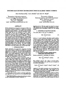
(a) (b) Fig.1. Experimental results of sequence ‘Bus’ supporting the two basic assumptions. (a) and (b) verifies Assumption 1 and Assumption 2 respectively.
All the experiments below are taken with JSVM 4.0 [3] under the spatial or the combined test condition proposed by [10], except that the base layer is not AVC-compatible. Firstly, experiments are performed under the spatial condition to demonstrate that the two basic assumptions mentioned in Section 2.2 are dependable. At first, we test the original JSVM encoder as an anchor and a simulcast encoder where no inter-layer prediction is utilized. Fig.1 (a) shows the coding efficiency results of the sequence ‘Bus’. Comparing the two RD curves at the same QP, the PSNRs are sufficiently close though the bit-rates are apparently different. This result supports Assumption 1. Then we test the original JSVM encoder as an anchor, and a changed encoder which disables inter-layer prediction for key frames, i.e. IPPP frames, on the CIF layer. Fig.1 (b) shows the number of output bits on each frame in the first GOP on the CIF layer of the sequence ‘Bus’. As expected, the changed one outputs more bits on frame 0 and frame 32, which are key frames. Whereas, on all other frames, the two schemes produce almost the same number of bits, including frame 16, which uses frame 0 and frame 32 as reference pictures directly. This result indicates that Assumption 2 is appropriate.
Sequences QP on the QCIF Layer QP on the CIF Layer QP on the 4CIF Layer α
Bus 30.0000 32.0000 1.03
Mobile 31.3686 34.3905 1.03
City 25.4337 27.5167 30.4004 1.01
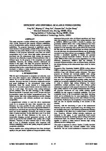
Fig.2 (a) and Fig.2 (b) show results of the sequence ‘Bus’ under the spatial and the combined condition respectively. A gain about 0.5 dB is reported in the case without MA, and the loss in the case with MA is about 0.1 dB. The lowest point on the curve of SIP with MA under the combined condition loses so obviously due to the drifting effect when the extractor cannot allocate enough bits to the QCIF layer. Fig.2 (c) shows the result of the sequence ‘Mobile’ under the combined condition. A gain up to 1 dB can be achieved, while the loss is less than 0.1 dB. Besides QCIF-CIF experiments, we also take QCIFCIF-4CIF ones. Fig.2 (d) shows the result of the sequence ‘City’ under the combined condition as an example. The gain is about 0.5 dB and the loss is about 0.05 dB.
Bus CIF 30Hz (spatial, α=1.03) 34 33.5 33 PSNR_Y (dB)
Table 1. QPs used in the spatial condition to obtain the SIP decisions.
[5] “Applications and Requirements for Scalable Video Coding,” ISO/IEC JTC1/SC29/WG11 N6880, Hong Kong, China, Jan. 2005. [6] K. Zhang, J. Xu, F. Wu, “Selective Inter-layer Prediction,” JVT-R064, 18th Meeting, Bangkok, Thailand, Jan 2006. [7] I. Amonou, N. Cammas, S. Pateux, S. Kervadec, “Coding rate coverage extension with dead substreams in the SVM,” ISO/IEC JTC1/SC29/WG11 M11703, Hong Kong, China, Jan. 2005. [8] A. Gersho and R. M. Gray, Vector Quantization and Signal Compression, Kluwer Academic, Norwell, MA, 1992 [9] T. H. Cormen, C. E. Leiserson, R. L. Rivest, C. Stein, Introduction to Algorithms, MIT Press, Cambridge MA, Sep. 2001. [10] M. Wien, H. Schwarz, “AHG on Coding eff & JSVM coding efficiency testing conditions,” JVT-Q009, 17th Meeting: Nice, FR, Oct, 2005.
32.5 32 31.5
anchor
31
SIP with MA
30.5
SIP without MA
30 300
400
500
600
700
800
900
Bit-rate (kbps)
(a) Bus CIF 30Hz (combined) 33 32.5 32 PSNR_Y (dB)
Secondly, experiments show that SIP improves coding performance on the high spatial layer in the case without MA, while keeping the loss very little in the case with MA. The original JSVM encoder is still chosen to be an anchor. In the SIP decision algorithm, we select Rmax = αRanchor. Although the SIP decision result is obtained under the spatial condition, it can also be adopted under the combined condition. The QPs and αs which are used under the spatial condition to obtain the SIP decisions for SIP coding under the combined condition are listed in Table 1. We select those QPs so that the bit-rates of bitstreams under the spatial condition equal to the highest bit-rates of bit-streams under the combined condition.
31.5 31 30.5
anchor
30 29.5
SIP with MA
29
SIP without MA
28.5 300
400
500
600
700
800
900
Bit-rate (kbps)
(b) Mobile CIF 30Hz (combined) 31 30.5
In this paper, a selective inter-layer prediction technique is presented. By disabling inter-layer prediction on some frames, the proposed scheme can obtain remarkable gains in the case without MA as well as keep the loss unapparent in the case with MA. Theoretically, how to select inter-layer prediction can be modeled as a 0-1 knapsack problem and can be solved by an algorithm based on dynamic programming. Experimental results show that, using the SIP method, coding gains can measure up to 1 dB in the case without MA and the loss in the other case is about 0.1 dB.
5. REFERENCES [1] “Joint Draft 5 with proposed changes,” JVT-R202-2, 18th Meeting, Bangkok, Thailand, Jan. 2006. [2] ITU-T, “Recommendation H.264,” http://www.itu.int/rec/T-REC-H.264200503-I/en, Mar. 2005. [3] “Joint Scalable Video Model JSVM-5,” JVT-R202, 18th Meeting, Bangkok, Thailand, Jan. 2006. [4] G. J. Sullivan, T. Wiegand, “Rate-Distortion Optimization for Video Compression,” IEEE Signal Processing Mag., vol. 15, pp. 74-90, Nov. 1998.
29 28.5
anchor
28
SIP with MA
27.5
SIP without MA
27 200
300
400
500
600
Bit-rate (kbps)
(c) City 4CIF 60Hz (combined)
PSNR_Y (dB)
4. CONCLUSION
PSNR_Y (dB)
30 29.5
36 35.5 35 34.5 34 33.5 33 32.5 32 31.5 31 30.5
anchor SIP with MA SIP without MA 700
900
1100
1300
1500
1700
1900
2100
Bit-rate (kbps)
(d) Fig.2. Comparison of coding efficiency. (a) is acquired under the spatial test condition and (b)-(d) are obtained under the combined test condition.