SELF LOCALIZATION OF MOBILE ROBOTS IN INDOOR ENVIRONMENT Giuseppina Gini , Francesco Amigoni, Andrea Bonarini, Vincenzo Caglioti, Marco Somalvico PM-AIR, Department of Electronics and Information, Politecnico di Milano, piazza L. da Vinci 32, 20133 Milano, Italy1 Phone Int +39 02 23993626, Fax Int +39 02 23993411, E-mail:
[email protected]
Abstract: The self localization of mobile robots in unknown environments is here approached trough the construction of maps based on sensors and recognition of natural landmarks. Our integrated navigation system replicates some functions of natural systems as using little a-priori knowledge, and using only sensors and camera on board. New images dynamically grow a map, constructed with simple mathematics and heuristics. In the first system presented we rely only on passive vision from a single camera. In the second we exploit a particular image deformation to obtain a complete view . Then we explore the use of laser pointing for mapping. The use of more robots in the exploration and map building is also developed. Keywords: autonomous robot, self localisation, mapping, computer vision
1. INTRODUCTION We want robots to be able to navigate autonomously in an unknown environment, using as the principal source of data a vision system. A single camera can solve problems in an indoor environment, when the robot moves on a plane surface. Visually guided systems often use artificial landmarks, while more advanced ones rely on natural landmarks. The self-location problem is important when the robot has to move in autonomous way. Dead reckoning reduces the location error, but is unable to keep the error under a given threshold. When used in telecontrol the self location is again important: the robot starts from any position, builds a map with any origin, and has to match the new map with the standard one shown in the user interface [Anousaki and Kyriakopoulos, 1999, Thrun, 1998]. Autonomy in a moderately dynamic system using vision is here developed with new algorithms based on the use of a single camera. The map is constructed from image interpretation, and computing the transformation from a local to a global map solves auto localization. The same approach is developed with data arising from laser pointing, with the difference that the segmentation gives results less ambiguous than in camera images.
Finally we give theoretical results in a system where more than one robot cooperate in mapping and navigating the environment. The important aspect of all our approaches is that they rely on natural landmark, and are suitable for application also in urban environments. Moreover, all the algorithms will improve their performances in a parallel architecture both for the classical image analysis step than for the mapping step that involves a high number of comparisons. In Section 2 we illustrate the first system, making use of a single camera pointing at the floor. The main problem here is the recognition of partial maps seen during the navigation as part of the global map constructed through exploration. In Section 3 we introduce the techniques used with special mirrors to see all around the robot. The problem here is to study the geometric properties of the images to find landmarks and obstacles. In Section 4 we introduce the techniques of mapping with laser beams. In Section 5 the multi-robot system is illustrated.
2. FROM FLOOR IMAGES TO MAPPING AND LOCALIZATION Our experimental set-up includes a Robuter, a PC, and a colour camera. The Robuter® is a mobile robot with differential drive. The on-board computer executes the motion commands and communicates at 9600 baud through a serial link with a PC. A sonar belt is integrated. The camera is
from Sony, PAL standard, with 768 columns of 512 pixels, is fixed and pointing to the floor. Matrox Meteor frame grabber is used in single acquisition. The flowchart of the global system is in Fig. 1. Image acquisition
start
no orthogonal axes, we build the K transformation from frame image to frame geometric-image:
1 K = 0 0
a *α a 0
u0 v0 1
(2)
The transform from scene to image is so: u' f v' = K * 0 w' 0
Analysis and floor search
0
0
f 0
0 1
x 0 y 0 * H * z 0 t
(3)
We can multiply the 3 matrices and obtain M:
x x u' m1 m2 m3 m4 y y v' = m5 m6 m7 m8 * = M * z z w' m9 m10 m11 m12 t t
some floor? No yes Map modification
Planning of the possible path
New goal definition
Path found? ? No yes move for a step the robot in the given direction
Figure 1. The flowchart of the system.
The strong points in our work are: Floor analysis and obstacles detection in single-camera images • New reduced calibration algorithm • Map creation using only visual data • Self-localisation as maps matching.
•
2. 1 Camera calibration To find the correspondence between real and image coordinates we developed a calibration procedure. We chose the pinhole model to compute world coordinates from image coordinates and the focal distance (f) through H. u' f v' = 0 w' 0
0 f
0 0
0
1
x x 0 y y 0 * = H * z z 0 1 1
(1)
To account for real problems as the position of the principal point, the aspect ratio, the α angle for
(4)
To calibrate the camera (estimating the 11 elements of M) we work in two phases: first from image to floor, then from floor to robot. The robot reference system has the origin in the middle of the axis connecting the operated wheels, and the orientation is forward. In the first calibration phase the camera takes a picture of a calibration object whose dimension is known (a white square, 21-cm width), and the vertex coordinates are computed. We choose all the points of the calibration object to be on the floor (z is null, and 3 elements of M are null). The initial estimate of M is done using least squares to match the reference square, then with Newton method. The reference system so constructed is on the floor and robot independent. Then we construct the matrix to transform it into the robot reference. During this second calibration phase, pictures of the object are taken from different positions and orientations of the robot, and the minimization is solved as before. Let x be the coordinate vector on the ROBUTER, ~ x the vector of the point in the image, f the function computing the floor point in the reference computed in the first phase, T the matrix to estimate.
x = T * f (~ x) a c T= 0 0
(5)
b 0 h cos(α) sin(α) 0 ∆x d 0 k −sin(α) cos(α) 0 ∆y = 0 1 0 0 0 1 0 0 0 1 0 0 0 1 To solve on the unknown α , ∆x , and ∆y (as in Fig. 2) we define a function which uses M and the available estimation of T to project the image points in the world points and compute the distance. The distance is then minimized
α
Figure 2. From the reference system on the floor to the robot reference system
A point in Cartesian space can be transformed into pixel coordinates u and v using: x u' y −1 v' = M * T * 0 w' 1 u' u= w' v' v= w'
(6)
For the reverse transformation,
(v * m9 − m5) * (m4 − m12 * u ) u * m9 − m1 S= (7) (v * m9 − m5) * (m2 − u * m10) + v * m10 − m6 u * m9 − m1 (m2 − u * m10) * S + m4 − m12 * u D= u * m9 − m1 m8 − v * m12 −
fx =
∑ red , green , blue
µ_ red( x, y) = m _red(x,y) =
( i, j) ∈Ι ( x, y)
and
N (red(i, j) − µ_ red(i, j))4 ∑ N
(9)
(N # pixels in the region)
∆ x∆ y
(3 −
∑ red(i, j)
(i, j )∈Ι(x ,y )
moment ( x , y ) ) moment _ max 3
S x' x x' z' D and get y' = T * and y = y' (8) 0 z' z' z 0 1 The calibration problem is solved.
2.2 Image analysis The basic hypothesis is that the floor has a uniform texture. Using statistical analysis we can extract from the picture of the floor the areas occupied by obstacles because they change the regular pattern [Ayache, 1991, Horswill, 1993, Mirmehdi and Petrou, 2000]. Since the image is in RGB format, for each pixel the algorithm computes the mean and the 4th order moment for each of the RGB components of the pixel. The formulas for the red component are:
The 4th order moment is significant because it measures the disparity of the pixels: it has low values in uniform areas, high when there is a sharp change, as when an obstacle is seen on the floor. To reduce computations the average and the moment are not computed for every pixel but for a subset of uniformly distributed pixels and by linear interpolation for the other pixels. After computation a new image is created with new components for pixels constructed according to mean and moment for each colour. The new image is then transformed in HSL format, filtered and transformed in binary, removing the obstacles. This requires choosing a dynamic threshold based on a little square region in the bottom part of the image used as example of the floor. In Fig. 3 we see an example The formulas to compute the dynamic threshold for L and H are constructed adding a static component and a dynamic component modified by a filter. The static and dynamic parameters are manually set and depend on the floor texture and on illumination conditions. The function filter is: (3 − fx =
moment(x, y) ) moment _ max red,green,blue
∑
(10)
3
Reference zone
Figure 3. An example.
2.3 Mapping and path planning The map is a grid map, with square cells initialised to a mean numeric value. The value represents how much the robot “trusts” in the cell classification defined as free, obstacle, or unknown. Whenever the cell is seen again as free its vote is increased, if occupied is decreased. The value is a vote, which can filter also moving obstacles because temporary obstacles do not affect too much the value of a free cell. The size of the grid cell is chosen considering the needed
performances: using the Robuter, cells with a side of 5cm give very good results. Using the parameters obtained from camera calibration, the binary image is mapped on the floor plane and added to the map, in a position obtained using the estimated pose. So, the map is created and enlarged after every image analysed. The map generated from the obstacle in Fig 3 is in Figure 4, where the lighter area represents free space, the darker cells represent obstacles, the black are unknown, and the grey not yet allocated.
comparison is mainly based on the angles between the walls. The robot can upgrade its location matching the global and the local maps. Complete map Mappa completa dell’ambiente
Position of the second map
y
x
Reconstructed partial map
y
Figure 4 The map resulting
To create a new map we assign the start position and a destination. To reach the destination the robot will explore the world, looking at the floor and generating obstacles. Every time a new obstacle is detected, the robot computes the path to reach the destination, and the map grows. To map the entire environment it will be enough to give as goal location a position unreachable, as outside a wall. Using the map the robot can navigate autonomously in the environment towards a specified goal pose. The path is found with A* on the visibility-graph of expanded obstacles [Latombe 1991]. Obstacles are enlarged by the half of the robot-width, not considering its length; in fact the robot moves forward and keeps obstacles on the sides. To allow the robot to move in narrow corridors with curves, the obstacles are enlarged and also smoothed. In this way, the robot can pass through very small passages, only a few cm wider than the robot. However, not considering the robot length implies that we have to take care of possible frontal collisions with obstacles; this is avoided by using sonar. In the same way highly dynamic obstacles are avoided just stopping in front of them and switching to another path.
2.4 Self-localization When the robot has a complete map of the environment, it can auto-localize itself. To do this, it creates a new map, starting from scratch, and compares it with the complete map. The
x
Figure 5. Matching
So the problem of matching a partial map onto a complete map, as in Fig 5; is based on the angles characterizing obstacles: in indoor environments usually they are 90°, or 180°. Starting from vector quantization we individuate segments having a common vertex. The map matching will find the correspondence (position and orientation) of the partial map in the global map using a vote system. Each local angle is matched against all possible global angles and the rototraslation matrix is computed. Every match generates a hypothesis of positioning of the local map. Each hypothesis has an associated vote (weight): − amplitude1 − amplitude2 180 weight = 10 * e
(11) with the maximum for same amplitude angles. The real position has a high vote, since all the angles are correctly matched. To reflect on the model the imprecision about data we associate a gaussian with maximum equal to the vote to every position. Summing up all the Gaussians we obtain a surface with a maximum in the position where the probability to find the robot is maximum, as in Fig. 6. The search for maximum is done considering that the number of local maxims is the number of the gaussians. Gaussians are represented in an array, every cell initialised to the weight of the respective hypothesis. Each maximum is moved to
the nearest cell containing a greater value of weight. When no more cells have a greater value the considered hypothesis is the local maximum. The global maximum is found and gives x and y. To find the orientation we use the orientation information associated to the hypotheses. 40 35 30 25 20 15 10 5 0 0
3,00
10
20
30
40
2,50 2,00 1,50 37
1,00
31
0,50
25
37
29
7 33
21
25
13
13 17
1
19 5 9
0,00
1
Figure 6. Four hypotheses and their gaussian representation.
robots equipped with this type of sensors can exchange information with robots equipped with other sensors for cooperative localization.
3.1 The sensor Omnidirectional vision makes it possible to cover a 360 degrees field of vision, by analysing only one image. This makes it possible to implement fast vision sensors suitable for a wide range of applications, such as: surveillance, robot (and vehicle, in general) navigation, tracking. In this section, we present our omnidirectional vision system. Our vision system is based on a camera facing upwards beneath a mirror. We have used different types of mirrors. We discuss here only results obtained by a conical mirror [Yagi et al., 1994] and a multi-shape mirror [Bonarini et al, 2000] obtained by the intersection of a truncated cone and a sphere. The environment surrounding the robot reflects in the mirror and the camera takes an image that contains information about what is surrounding the robot. The conical mirror gives an image like the one presented in Figure 8, taken in a corridor. The radial lines correspond to vertical edges in the environment.
To improve this algorithm, for each local maximum the program increases the vote of the associated position if this position matches two segments in the maps. The matching is confirmed only when • The angular difference is less than a threshold • The centroid distance of the segments is less than half of the greater segment • The maximum distance of the segments is less than a threshold. The final weight is so computed in (12) − amplitude1 − amplitude 2 − max_ dis tan ce 1 K K2 weight = K * e *e
(12)
which gives a low weight to segments far away and with different amplitudes. In this way only the correct position gets a high vote.
3 SELF-LOCALIZATION WITH OMNIDIRECTIONAL VISION SENSORS In this Section we introduce a panoramic vision [Benosman, Kang, 2001] sensor [Bonarini, 2000][Bonarini et al. 2000][Lima et al., 2001] covering the 360 degrees field of view around the robot (omnidirectional vision). We will also discuss how it can be used to support selflocalization. In the next section we will see how
Figure 7. The omnidirectional sensor with the conical mirror.
We have designed the multi-part mirror with the specific aims of covering the widest area around the robot, while maintaining enough resolution on the far area to be able to identify the smallest interesting object in the environment with minimal resolution of 1 pixel/cm. At the same time, we can recognize objects close to the sensor. These requirements cannot be matched by the classical shapes used for sensors of this kind [Yagi, Kawato, Tsuji, 1995] [Benosman, Kang, 2001]: cone, sphere, hyperbole, parabola.
3.2 Localization of an object with the omnidirectional sensor
Figure 8. An image taken by the conical mirror in a corridor.
We have started by considering a cone-shaped mirror, which was immediately discarded because of the strong distortions it introduces in the image. A benefit of this mirror shape lies in the possibility to select the pan angle to obtain a wide field of vision at will. Working with a spherical mirror, we have noticed that it does not modify too much the shape of objects, but a large percentage of the image is useless because it contains the chassis of the underneath robot. With this system we have obtained a vision field ranging more than 5 m in any direction, but the resolution of the image obtained in this way did not match the specifications. Therefore, it has been necessary to find a trade-off between the bend radius of the mirror and the height where it was placed, avoiding an excessive reduction of the vision field, or its exaggerated opening with drastic reductions of the resolution. We have designed a mirror composed of a sphere intersecting a reversed cone. This shape allows exploiting the characteristics of the spherical mirror to a distance of 2 meters, so the objects that fall in this range are not much deformed and have a satisfying resolution. The objects at a distance greater than 2 meters are reflected in the conical part of the mirror, designed to allow the identification of objects at a distance up to 6 m with sufficient resolution. A typical image taken from the multipart-mirror is in fig. 9.
For localization purposes, only vertical edges in the environment (radial edges on the image) are considered. We have developed optimised algorithms to detect these edges, whose position is estimated with an error of about 2% in distance and ±1 degree in position. Self localization is based on triangulation on the most characteristic edges, selected on the basis of their position, their reliability, and their persistence in time, during the movement of the robot. Knowing the angular and linear speed of the robot [u(t),v(t)], let us consider an object (in our case an edge) P whose position at time t1 is P1 ( X1 , Y1 , Z1 ) and whose relative speed at time (t1 + t ) are [ − u(t1 + t ),− v (t1 + t ),0 ]. The position of P at time (t1 + t ) is given by [Yagi, 1995]: t
XP = YP =
∫ − u (t
1
t=0 t
∫ − v (t
t =0
1
+ t )dt + X 1
+ t ) dt + Y1
Z p = Z1
(13) (14) (15)
Since the relationship between the θ and the position oP is:
tgθ =
Yp Xp
(16)
it is possible to obtain the relationship between the azimuth and the position of an object at time t1+t as: t
∫ − v(t
1
tgθ (t1 + t ) =
+ t )dt + Y1
t =0 t
(17)
∫ − u (t
1
+ t )dt + X1
t =0
Knowing the azimuth θ in two subsequent images, it is possible to find the position of the object with respect to the robot by triangulation: −1
X1 tgθ 2 −1 V (2) −U (2)tgθ 2 Y = tgθ −1 • V (3) −U (3)tgθ (18) 1 3 3 tgθ 2 ≠ tgθ 3 For i in {2,3}: t
U (i ) =
∫ − u (t1 + t(i)) dt
(19)
t=0 t
V (i) = Figure 9. An image taken in a heat production plant.
∫t =0− v(t1 + t (i))dt
(20)
where θ 2 and θ 3 represent respectively the azimuth θ after a time t 2 and t 3 .
3.3 Self-localization with the omnidirectional sensor The triangulation method proposed above may have some problems due to imperfect knowledge of the elements used to localize edges in the environment. We have faced these problems by filtering techniques and heuristics used to select the reference edges. Let us discuss these first. We only consider edges that can be tracked for enough time while the robot is moving. Among them, we select a set of relevant edges basing on the following considerations. Since the precision of the localization is higher for closer edges, these are preferred to more distant ones. Since localization of the object has higher quality when the position of the object detected in two subsequent time points is higher, lateral edges are preferred to edges in the direction of movement of the robot. Moreover, we consider a set of reference edges evenly distributed in the azimuth space, so to reduce systematic errors. A sort of Kalman filtering is done on the track of each edge in time. If the robot is not rotating with respect to the tracked edge, this follows an arctg curve in time. We estimate the expected position of the tracked edge at a given time, and correct the estimate as the robot proceeds, by
considering also the information coming from the other tracked edges. In Figure 10, we show an example of the edge tracks. In the right top part of the figure we have represented a robot (the hatched rectangle with a circle in the middle) moving with respect to an object from position A to positions B and C. In the lower part of the figure we see the plot of the azimuth values for the edges detected by the sensor on the robot, during time. At each instant, the azimuth values detected are associated to an edge already detected, or to a new edge, as it happens at point B, where edge number 4 becomes visible. The shape of the plot can be estimated and expectations can be generated.
4. FROM POLAR RANGE SENSOR MAPS TO SELF LOCALIZATION The general problem we address here is to localize a robot equipped with a laser polar range sensor. A laser polar range sensor measures the distance between laser origin and the objects in the surrounding environment along several rays (at a fixed height from the floor). The rays sweep an angle of 180 degrees in front of the robot and are equally spaced every 0.5 degrees.
A
C
B
x
y
1
ϑ 4
2 3
3,2,1
2,1
2,1,4
1,4
0°
-9 0 °
A
B
C
Figure 10. A sample movement and the respective edge tracks.
time
The points acquired from a scan are transformed in a set of lines called partial map. The devised localization method is actually independent from the sensor that perceives the partial maps provided that they are sets of segments. The localization method integrates two partial maps called M1 and M2. The method is composed of two major steps: • find possible transformations of M2 on M1; • evaluate every transformation to identify the best match between M1 and M2. We note that the partial maps are the result of the perception activities of a single robot in two different locations. They can as well be the result of perception of a pair of robots in two different locations. Let us start by the first step: how to find possible transformations. The partial maps are analysed in order to extract the landmarks that can play as basis to integrate the partial maps together. We use corners as landmarks. A corner is an angle formed by two segments. A transformation is a roto-translation that brings at least one angle of M2 (say α2) on an equal angle of M1 (say α1). A transformation is thus a triple . (Xt, Yt) is the translation needed to move the vertex of α2 on the vertex of α1. θr is the rotation to move one line of α2 on the same direction of the corresponding line of α1. The rotation is centred in (Xr, Yr) that is the vertex of α1. For each partial map, we look at all angles formed by segments in the map. On the basis of these angles all the possible transformations are generated. The second step is the evaluation of the transformations. Every transformation found in the previous step is evaluated to find the best one. To find the measure of a transformation t we move M2 on M1 according to t, then we evaluate the approximate length of the segments of M1 that match with segments of M2. Thus, the measure of a transformation is the length of corresponding segments. Once the best transformation tb has been found, the second partial map M2 is transformed to the reference frame of M1 according to tb. In this way, the point P corresponding to the origin of M2 in the reference frame of M1 gives the position of the robot while taking the partial map M2. Thus, a localization of the robot based only on the geometrical feature of the environment id obtained. The described method calls for an implementation on a parallel computer. For example, the process of evaluating the possible transformations is composed of a number of
similar activities, namely evaluate a transformation, that operate on different data and that can be conveniently distributed over the processors of a parallel computer. This could improve the performance of the system with respect to the sequential evaluation of the transformations on a single processor. The experimental results of the method are now described. The quality of the partial maps acquired by the mobile robot in an environment heavily depends on the type of environment: corridors are mainly composed of long “good” segments, open spaces and offices are mainly composed of a mess of short “bad” segments. The partial maps used in the experiments have been taken by the robot at locations where the robot was manually driven. The distance between two successive origins of scan is about 1 meter. This value has been experimentally determined, since we notice that with distance between scans greater than 1.5 meters the integration rarely succeeded (because the two partial maps have only a small common portion where it is difficult to find good angles for transformation). It is too expensive to find and evaluate all the possible transformations between two partial maps. In fact, there can be n12n22 possible transformations, where n1 and n2 are the numbers of segments in M1 and M2, respectively. Moreover, only few of the possible transformations are significant, namely bring the two partial maps in a reasonable position. It is obvious that the fact that a transformation is significant can be discovered only when it is evaluated. We have used four possible methods for finding a set of significant transformations between the two partial maps. The methods adopt different techniques to identify the angles on which transformations are based. Angles Between Successive Segments. For each partial map, we look only at angles between two successive segments. The method proceeds in two parts: finding the angles in the partial maps and finding the transformations between them. We note that the first part of the algorithm heavily relies on the assumption that the segments in M1 and in M2 are ordered in some way. Angles Between Randomly-Picked Segments. For each partial map, we look at angles between two segments that are randomly picked up among the most significant ones. In order to do this, we assign high probability to be picked up to longest segments, since they carry the most precise information. The method tries first to transform M2 on M1 according to angles between longest (randomly selected) segments. If it is not possible, or if the best obtained match is not good enough,
the algorithm considers shorter and shorter segments to find a transformation that gives a good match. Angles Between Perpendicular Segments. For each partial map, we look at angles between segments that are perpendicular. This method is convenient for indoor environments, where the presence of walls usually produces perpendicular segments. The method is based on the creation of histograms. The histogram of M1 (and, in similar way, that of M2) is an array with a number of elements equal to the number K of buckets in which the possible orientations of segments (from 0 to π, with respect to a fixed axis) are divided. Each element Li of the histogram of M1 is the list of segments of M1 with orientation (relative to a fixed axis) between π/K*i and π/K*(i+1). To each element Li of the histogram of M1 is associated a value: the sum of the lengths of the segments in Li. The principal direction of a partial map is defined as the element of the histogram with maximum value. The normal direction of a partial map is defined as the element of the histogram that is π/2 away from the principal direction. All Transformations. For each partial map, we look at all angles formed by segments in the map and generate all the possible transformations. Each scan is usually composed of a number of segments ranging from 20 to 100, according to the kind of environment. The possible transformations for a pair of scans range from one hundred to some thousands, depending on the method selected and on the number of angles in the scans. The time required carrying on the whole process of integration of two partial maps range from few seconds to dozens of seconds on a 700MHz Pentium III processor. The proposed method is robust with respect to changes in the environment in which the robot is localizing itself. For example, in Figure 11, in the first partial map there is a partially open door (left side) while during the scanning of the second partial map (the door was closed. The method finds the correct integration as in Figure 12.
Figure 11. Mapping with a door: open or closed.
Figure 12. Final map
5. COOPERATIVE LOCALIZATION OF MULTI-ROBOT SYSTEMS In this Section, we propose a framework for the cooperative localization of a system consisting of n mobile robots. Many results are available on the self-localization of single mobile robots (e.g., [Fox et al. 1998, Borghi, Caglioti 1998]). Recently, attention has been focused towards to multi-robot localization: in the work of [Thrun et al. 1999] only partial information is maintained (the socalled factorial representation) about the pose of the robots. In this section, complete information about robot pose is maintained and updated through an efficient distributed process: this is made possible by adopting Gaussian distributions for the involved parameters. In this framework, there is no need for any centralized agent: each single mobile robot is equipped with one or more sensors (no central sensor exists). In addition, the localization is performed by updating a current estimate of the
robot poses in correspondence of each sensor measurement: to update the current estimate, the robots communicate with each other and update locally stored information: again, no central site exists, where the whole pose information is stored and maintained. The map of the robot environment is supposed to be known, modulo moving obstacles. Each robot i perform sensor measurements, which can be aimed either at the environment or at another mobile robot j. It is shown that, under broad hypotheses, the problem of maintaining and updating pose information is scalable, i.e., the time and space needed for updating the estimate at each of the n mobile robots is of the order of 1/n of the time and space that would be needed for update the estimate of the robots by a centralized agent. The following hypotheses are assumed: • the pose estimation errors and the measurement errors are supposed to be mutually gaussian; • the pose estimation errors are kept small enough (e.g., by dead reckoning), such that the relationships between errors in the different parameters can be well approximated by linear relations; • the computational cost for broadcasting a datum from a single robot to the remaining ones is O(n). First, let us calculate the space complexity and the time complexity of updating the pose estimation of n robots by means of a centralized agent within the above described gaussian framework. To correctly update pose estimates, both the pose estimates and the self- and mutualcorrelations must be maintained and updated. This requires O(n2) time using O(n2) storage, in correspondence to each sensor measurement. This process is described by the Kalman estimator (1) below. By using measures related to the relative positions between robots (or between a robot and the environment), the pose estimate updating problem is shown to be scalable: the estimate update corresponding to each sensor measurement can be performed in O(n) time by distributing the process among the n robots. In addition, each robot only needs to maintain O(n) data in its memory. Now we consider a system consisting of n mobile robots, which navigate within a known environment. In order to maintain an estimate of the pose of the robots, each robot performs a sensor measurement aimed either at the environment or at another robot. Once such a sensor measurement has been performed, the measuring robot updates its pose estimate and the
correlation between its pose and the pose of the other robot, and it propagates the information towards the remaining robots, which in turn update both estimate and correlations. Let x i = [ X i Yi ϑi ]T be the vector of the pose parameters of the mobile robot i, where [ X i Yi ] are the coordinates of the origin of a reference attached to the robot i, while ϑi is the orientation angle of the abscissa axis of this reference. T
... x n ] T Let x = [ x1 indicate the column vector formed by the pose vectors of the n mobile robots. T
T
... x n ] T the Let us indicate by x = [ x1 vector collecting the current estimates of the poses of the robots. Let Σ ii indicate the 3 x 3 covariance matrix of the pose parameters of robot i, and let Σ ij indicate the correlation matrix between the pose parameters of robot i and the pose parameters of robot j The covariance matrix of the pose vector x is given by T
Σ11 Λ=
... Σ 1n
... ... ... Σ n1 ... Σ nn
Suppose that a measurement z is taken, whose result depends on some of the poses x i : the linearization of the relationships between z and x can z = H x + w, where w is a measurement error, which is supposed to be independent of x, and H is the Jacobian matrix of z with respect to x. If σ 2 is the variance of the error w, the a posteriori Kalman estimate of the pose parameters, and its covariance matrix are given by: xˆ = x + ΛH T ( HΛH T + σ 2 ) −1 ( z − Hx ) Λ ' = Λ − ΛH T ( HΛH T + σ 2 ) −1 HΛ
(21)
Now consider the case where the measurement z only depends on the relative pose between robot i and robot j: from z = hi x i + h j x j + w the expression of H becomes
H = [0 ... 0 hi the expression of ΛH
T
0 ... 0 h j becomes
0 ... 0]
σ 1i hi + σ 1 j h j T
T
σ h + σ 2 jhj ΛH = 2i i ... T T σ ni hi + σ nj h j T
T
T
and the expression of HΛH T becomes: H Λ H T = hi Σ ii hi + 2 hi Σ ij h j + h j Σ jj h j (22) With these expressions, the a posteriori estimates of the poses of the mobile robots are T T T T xˆ k = xk + (Σkihi + Σkjh j )(hiΣii hi + 2hi Σij h j T
T
T
(23)
+ h j Σ jj h j + σ 2 ) −1 ( z − hi xi − h j x j ) while the a posteriori self-correlations are T
Σ kk ' = Σ kk − (Σ ki hi + Σ kjh j )(hi Σ ii hi + 2hi Σ ij h j + T
T
T
T
h j Σ jj h j + σ 2 ) −1 (hi Σ ik + h j Σ jk ) T
(24)
and the a posteriori cross-correlations are
Σ kl ' = Σ kl − (Σ ki hi + Σ kjh j )(hi Σ ii hi + 2hi Σ ij h j + T
T
T
h j Σ jj h j + σ 2 ) −1 (hi Σ il + h j Σ jl ) T
T
(25)
All these expressions can be locally calculated by any single robot, using an O(n) storage, in O(n) time. In fact, the following information is propagated from the measuring robot i to the other ones: the term (2), hi , h j , xi , x j . These O(1) items only need O(n) time to be propagated to all robots. Each robot k can calculate expression (3) and (4) in constant time using O(n) storage, while a total O(n) time (using O(n) storage) is sufficient to calculate the n-1 updated cross-correlations (5): in fact the central factor in round brackets is immediately calculated from term (2), while the other factors are calculated by combining the broadcasted terms plus the locally stored terms Σ kl . The obtained result can be summarized by the following theorem: Theorem. Under the hypotheses illustrated above, the pose estimate updating process is scalable over the n robots: in correspondence to any sensor measurement, the global pose estimate can be updated in O(n) time using O(n) storage at each robot.
A preliminary implementation of the approach described in this Section has been carried on two mobile robots: one equipped with an orientable laser range finder, and the other equipped with an omni-directional vision sensor (COPIS). Both robots navigate within the hall of our Department, whose map is known. After a few seconds, any robot performs a sensor measurement, either aimed at the other robot, or aimed at the environment (according both to “visibility” conditions and to uncertainty criteria [Caglioti 2001]). After each sensor measurement, both robots update their pose estimate and the correlation matrix. An example is reported in Figure13, illustrating the estimate updating after Robot 1 performs a single range measurement with its laser range finder. The estimate update depends not only on the measurement result, but also on the current estimate and correlation matrix. It can be noticed how the global pose estimate improves by virtue of the sensor measurement: the apparently small estimate variation is due to the fact that a single parameter is measured (namely, the distance between the range sensor of Robot 1 and the surface of Robot2 along a certain direction) in comparison with the six parameters characterizing the global pose of the two robots.
6. CONCLUSIONS The unusual aspects of our integrated navigation systems are: simple design, efficient use of special properties of the environment, and large autonomy. Efficiency and reliability are due to various factors. The specialization of the environment allows the robot to reduce the vision computation. The use of simple reactive strategies reduces the risk of failures, because obstacle avoidance is always active. Finally, the environment does not need any modification to insert the robot. As illustrated in the previous sections, the uncertainty of the world is simply managed through heuristics and through a strict use of information only obtained through sensors. Our results confirm that solutions to the auto localizations are available in unstructured environments searching for natural landmarks.
Actual pose 4000
Odometric data
R o bo t 2 Updated estimate
R ob ot 1 y th e ta x A c tu al p o s e 4485 451 0. 29 O d om e tri c e s ti ma t e 4 4 9 8 4 7 3 0 . 1 2 U p da te d e s ti m a te 4488 457 0. 15 0 2000
6000
R o bo t 1
R ob ot 2 x y th e ta 3 976 2995 90. 3 A ct ua l p o s e O do m e tric e s tim a te 3 9 8 6 2 9 9 7 9 0 . 2 6 U pd a te d e s ti m at e 3 983 2996 90. 32
Figure 13: Updated estimates after a sensor measurement by Robot 1
REFERENCES [Anousaki and Kyriakopoulos, 1999] G.C. Anousaki, K.J. Kyriakopoulos. Simultaneous Localization and Map Building for Mobile Robot Navigation. IEEE Robotics & Automation Mag, September 1999, 42-53. [Ayache, 1991] N. Ayache. Artificial vision for mobile robots. The Mit Press, Cambridge, Massachusetts, 1991. [Benosman, Kang 2001] R. Benosman, S. B. Kang (Eds.) Panoramic Vision: sensors, theory and applications, Springer Verlag, Berlin, D. [Bonarini, 2000] A. Bonarini, The Body, the Mind or the Eye, first? In M. Veloso, E. Pagello, M. Asada (Eds), Robocup99 – Robot Soccer World Cup III, Springer Verlag, Berlin, 210–221, 2000. [Bonarini et al, 2000] A. Bonarini, P. Aliverti, M. Lucioni. An omnidirectional sensor for fast tracking for mobile robots. IEEE Transactions on Instrumentation and Measurement, 49, 3, 509-512, 2000. [Borghi and Caglioti 1998] G.Borghi, V.Caglioti. Minimum uncertainty explorations in the selflocalization of mobile robots in curvilinear environments. IEEE Trans. on Robotics and Automation, 1998. [Caglioti, 2001] V.Caglioti. An entropic criterion for minimum uncertainty sensing in recognition
and localization tasks: theoretical and conceptual aspects IEEE Trans. SMC,Part B, 2001. [Horswill, 1993] I. Horswill. Polly: A VisionBased Artificial Agent. Proc. AAAI-93, AAAI Press/The MIT Press, 1993. [Latombe, 1991] J.-C. Latombe. Robot motion planning. Kluwer academic publishers, Boston, 1991. [Lima et al., 2001] P. Lima, A. Bonarini, C. Machado, F. M. Marchese, C. Marques, F. Ribeiro, D. G. Sorrenti. Omnidirectional catadioptric vision for soccer robots. Int J of Robotics and Autonomous Systems, 36, 2-3, 87102, 2001. [Mirmehdi and Petrou, 2000] M. Mirmehdi, M. Petrou. Segmentation of color textures. IEEE Trans PAMI, Vol 22, n° 2, 142-159, 2000 [Thrun, 1998] S. Thrun. Learning metrictopological maps for indoor mobile robot navigation. Artificial Intelligence, 99, 21-71, 1998. [Thrun et al., 1999] D.Fox, W.Burgard, H.Kruppa, S.Thrun. A Monte Carlo algorithm for multirobot localization. Techn. Rep. Carnegie Mellon University, CMU-CS-99-120, 1999. [Yagi et al., 1994] Y. Yagi, S. Kawato, S. Tsuji, Real-Time omnidirectional Image Sensor (COPIS) for Vision-Guided Navigation, IEEE Trans R&A, 10, 1, 11-22, 1994.