Vision based Localization of Mobile Robots using Kernel ... - CiteSeerX

Vision based Localization of Mobile Robots using Kernel approaches Hashem Tamimi and Andreas Zell Computer Science Dept. WSI, University of T¨ubingen T¨ubingen, Germany Email: [tamimi,zell]@informatik.uni-tuebingen.de

Abstract— The aim of this article is to present the potential of Kernel Principal Component Analysis (Kernel PCA) in the field of vision based robot localization. Using Kernel PCA we can extract features from the visual scene of a mobile robot. The analysis is applied only to local features so as to guarantee better computational performance as well as translation invariance. Compared with the classical Principal Component Analysis (PCA), Kernel PCA results show superiority in localization and robustness in presence of noisy scenes. The key success of the kernel PCA is the use of fractional power polynomial kernels.

I. I NTRODUCTION The problem of robot localization can be classified as either global or local localization [10]. In global localization, the robot tries to discover its position without previous knowledge about its location. In local localization, the robot must update its position using its current data from its sensors as well as the previous information that it has already accumulated. The lack of any historical information about its surroundings makes the global localization more challenging [7]. The idea of feature based robot localization involves representing the robot environment as a topological map by means of a large set of features. The main properties of these features are: (1) They should be a compressed form of the original scenes so as to speed up the computation of the comparisons, still, they should maintain distinguishing representations of the scenes. (2) They should exhibit invariance against different transformations on the scenes such as translation and scale. (3) They should also exhibit robustness against noise or illumination changes, which the robot encounters during its navigation. PCA has been applied in the field of robot localization. In [5] active vision is combined with robot localization using PCA. In [1] and [13] the study of the problem of batch learning and the use of incremental PCA is presented. Their idea is to deal with on-line leaning of the robot landmarks without recomputing the PCA for the whole samples each time. The work done in [4] presents the effect of illumination on PCA. They present illumination invariant features by filtering the eigenimages rather than filtering the original samples. In [12] a comparison among different vision-based robot localization approaches is made. Their results show that PCA is more robust and accurate than other methods such as edge density based, but also show that PCA requires more computation power.

Robot localization using PCA can be classified as either local and global based on the feature extraction applied. In the global based approach [8], the whole image is considered as a sample and applied to the PCA as a vector. An example of global features is the work done in [3], where PCA is globally applied to panoramic images, they introduce robust PCA using an expectation maximization approach where outliers can be resolved. On the other hand, in the local based approach, a set of landmarks (small patches) are first selected from the image and transformed into vectors to be further handled by PCA [11]. PCA based methods have demonstrated their success in the field of robot localization as well as in face recognition, data compression, and many other applications. However, PCA is an appropriate model for data generated by a Gaussian distribution, or data best described by a second order correlation. It is well known, however, that the distribution of natural images is highly non-gaussian. Kernel PCA, originally proposed by Sch¨olkopf et. al. [9], was investigated as a generalization of PCA. While PCA aims to find a second order correlation of patterns, KPCA provides a replacement which takes into account higher order correlations. The success of KPCA is demonstrated in the area of image processing, such as face recognition, image de-noising, texture classification and other applications in other different fields. Another well known approach which has proved successful on classification problems is the Linear Discrimination analysis (LDA). This method fails for nonlinear problems and therefor was extended to a kernel based approaches in [Baudat] which is called GDA. The remaining sections of this paper are organized as follows: Section (II) reviews the KPCA and GDA approach for feature extraction and classification and also presents some commonly used kernels. Section (III) deals with the methodology of finding the landmarks in the images where features are to be extracted. In section (IV) we focus on the robot training phase. In section (V) we explain the process of localization after the robot is being trained. Section (VI) presents the test model used to measure the success of our localization experiments. In section (VII) we discuss the experimental results of our approach.

II. N OTATION

III. L ANDMARK S ELECTION

Kernel PCA can be derived using the known fact that PCA can be carried out on the dot product matrix © ªN instead of the covariance matrix [9][14]. Let xi ∈ RM i=1 denotes a set of data. Kernel PCA first maps the data into some feature space F by a function Φ : RM → F , and then performs standard PCA on the mapped data. Defining the data matrix X by X = [Φ (x1 ) Φ (x2 ) · · · Φ (xN )], the covariance matrix C in F becomes:

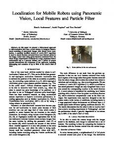
Our approach of robot localization is done using visual features. The features are extracted from the image using a model of visual attention like that used in [11]. We also adopt local features (landmarks) instead of global features for two reasons: (1) To reduce the computational time of the feature extraction done by Kernel PCA. (2) To benefit from the translation invariance nature of the local landmarks. We propose a two-phase approach: training phase and localization phase. Figure (1) shows the system components illustrating the different stages of each phase. In the training phase we assume that the robot would initially collect sufficient landmarks to represent the robot environment. It is important to understand that Kernel PCA employs batch learning in nature, this means it can not be applied until all the samples are ready. In the localization phase the robot should compare the features of the actual scene with the stored features. The result of such a comparison would lead to the knowledge of the robot position. The system components are discussed in details in the following subsections.

C=

N 1 X 1 T Φ (xi ) Φ (xi ) ≡ XX T N 1 N

(1)

We PN assume that the mapped data are centered: 1 Φ (xi ) = 0. We can find the eigenvalues and eigenvectors of C via solving the eigenvalue problem: 1 N

λu = Ku

(2)

The N × N matrix K is the dot product matrix defined by K = N1 X T X where:

N X

uhi k (xi , x)

Landmark detection Feature extraction Redundancy removal

Localization phase

yh = v h • Φ (x) =

Training phase

1 1 Φ (xi ) • Φ (xj ) = k(xi , xj ) (3) N N Let λ ≥ · · · ≥ λp be the nonzero eigenvalues of K (P ≤ N, P ≤ M ) and u1 , ..., uP the corresponding eigenvectors. Then C has the same eigenvalues and there is a one-to-one © h ª correspondence between the nonzero eigenvectors u of K and the nonzero eigenvectors © hª v of C : v h = αh Xuh where αh is a constant for normalization. have ° ° √ If both of the eigenvectors √ unit length, αh = 1/ λh N . We assume °uh ° = 1/ λh N so that αh = 1. For a test data x, its h-th principal component yh can be computed using kernel functions as: Kij =

Landmark detection Feature extraction Feature Comparison

Generalization

Label identification

Labeling

Localization

(4)

Database

i=1

Then the Φ image of x can be reconstructed from its projections onto the first H (≤ P ) principal components in F by using a projection operator PH PH Φ (x) =

H X

Fig. 1.

System Components

IV. T RAINING PHASE yh v h

(5)

h=1

Commonly used kernels include: ³ ´ kx−yk • Gaussian Kernel: k (x, y) = exp − 2σ 2 , • Sigmoid Kernel: k (x, y) = tanh (κ (xi , y) + Θ), d • Polynomial Kernel: k (x, y) = (x, y) . The polynomial kernel has three famous degrees: (d = 1) is the linear classical PCA, (d > 1) the polynomial kernel taking into account integer values, and (0 < d < 1) is the fractional power polynomial presented in [6]. In the following sections we concentrate mainly on the polynomial kernel. Results from some preliminary experiments that we made show that the polynomial kernel not only demands relatively low computation time, but also leads to better localization rate than the other kernels.

A. Landmark detection Landmarks are parts of the image which hold sufficient information about the image. Usually a small set of landmarks per image is needed. A model of visual attention is responsible for tracking a given landmark during the robot navigation. We adopt a model based on edge density [11]. Let E ∈ R2 → R2 be the output of an edge detector on the image I. The edge density D is the sum of E over a region of size Ω in the neighborhood of each element x ∈ R2 : a candidate landmark S is defined as a set of sufficiently interesting local maxima of D. Figure (2) shows a sample image, its corresponding edge density is in figure (3). 1 X E (xi ) (6) D (x) = xi ∈Ω kΩk

D. Feature labeling Labels are introduced as relations between Landmarks to images. It is important to consider the two different relations seen in figure (4). Each image holds a set of landmarks and consequently a related set of labels. Similar landmarks are represented as common labels (shared by two or more images). The relation between labels and features is 1 : 1 because we hold only unique features as explained in subsection (IV-C).

F1

L1

F2

L2

F3

L3

F4

L4

F5

L5

Fn

Ln

Im

Labels

Images

I1

Fig. 2.

Sample Image showing positions of Landmarks

Features

Fig. 4.

I2

I3

Relation between features, labels and images

E. Generalization

Fig. 3.

Edge density showing positions of landmarks in squares

B. Feature extraction Features are extracted from each landmark using Kernel PCA as explained in section (??). Before features are being extracted, the landmarks are vectorized. These landmarks currently hold values from the gray level image component only. The resulting features are temporary and should be examined by the next stages. C. Redundancy removal It is possible that landmarks found in different images are similar. This similarity can be discovered through the corresponding feature similarity. The redundancy should be eliminated in order to have a normalized relation between landmarks and images. This means that only different features are stored at the end. Consider a set of landmarks S1 ...SN are collected during the robot training phase. These were detected using the landmark detection approach in subsection (IV-A). Let F1 ...FN ∈ ∆ be the corresponding features extracted through Kernel PCA. The decision of adding a new feature Fa to the training set ∆ is based on the criteria kFi − Fa k > τ, ∀Fi ∈ ∆ where τ is a given threshold.

One important aspect in the robot localization work is to have generalized and robust features. Robust features can represent the corresponding positions under various changes, mainly caused by variations of illumination or noise. One way to accomplish this is to apply noise to the training samples before labeling takes place. The noise is applied to the each landmark Si using additive noise: Si = Si + gσ , i.e. sums an random value to the image value at each pixel where σ is the variance of the gaussian noise being added. It is worth comparing the labeling behavior of the Kernel PCA and PCA with the presence of such additive noise. Figures (5) and (6) illustrate the attempt of mapping the features to their corresponding images. These features are extracted from noisy landmarks. In figure (5) we use Kernel PCA and perform the labeling. It is clear to see that Kernel PCA has successfully labeled the images with the features linearly, where the first 15 features are mapped to the image 1 and the second 15 features are mapped to the image 2 and so on. On the other hand, figure (6) shows the results of using PCA. The relation between the images and features is not clear because the noise has affected the mapping. The linear operation between features and images can be accomplished in the case of PCA only in the absence of noise. V. L OCALIZATION PHASE In the localization phase, seen in figure (1), the robot acquires new (unseen) images and tries to find out its position. The landmarks of the new images are detected using the landmark detection approach in (IV-A). Then,

300

is kept minimum for all positions in the train set, where c1 , c2 and c3 are adjusted according to human perception taking into account that c3 À c1 , c2 . This model approximates the reality where two images would look different from each other if they are physically far from one another. This model is subjected to failures in case of highly similar environments, like two rooms which look alike but are separated by a long corridor. A localization success rate can be finally defined as

250

Label No.

200

150

100

50

0

0

Fig. 5.

20

40

60

80

100 Image No.

120

140

160

180

200

R=

Number of correctly localized scenes Total number of scienes

(9)

Kernel PCA labeling, using noisy landmarks

800

700

VII. E XPERIMENTAL RESULTS

600

We constructed a database of features that represent 200 different distributed positions. Each position has 15 candidate landmarks, taken from gray scale images. Each landmark is 15 × 15 pixels. For Kernel PCA [2], we investigated the approach using different degrees of the polynomial kernel and different number of eigenvalues. To test the ability of localization, we used another set containing 500 images located in the area around the trained landmarks. The images exhibit different transformations compared with the training images such as translation, scale, or rotation. We also studied the performance of the approach in presence of noisy images. As noise generation is done randomly, the experiments were done many times and the average localization rate was finally calculated. The results in figure (7) show the average localization rate of the test images based on equations (7) and criteria (8). It is clear that using a polynomial kernel of fractional degree leads generally to better results than using either PCA or an integer polynomial degree. The best performance is obtained when the degree is 0.8 where the localization rate reaches 86%. Figure (8) is a comparison between PCA and kernel PCA with a polynomial kernel of degree 0.8. We use different number of eigenvalues and calculated the average of the localization for each given eigenvalue. We only illustrate the part of study where the number of eigenvalues is between 5 and 15. Higher eigenvalues not only lead to lower localization rate but are also undesired because of the increasing size of the feature vector and because of their embracement of noise. Feature vectors of less than 5 values can hardly contain sufficient information. The figure shows that kernel PCA leads to better performance than PCA in each case. Finally, figure (9) demonstrates the capability of our approach to retrieve similar images to the image in the query. Color does not play any role in our approach, we use only gray scale images. The query images are in the first column at the left hand side, and the resulting images are sorted from left to right in accordance to the degree of similarity as in equation (7).

Label No.

500

400

300

200

100

0

0

20

40

Fig. 6.

60

80

100 Image No.

120

140

160

180

200

PCA labeling, using noisy landmarks

features are extracted from these landmarks as explained in (IV-B). Each new feature is compared with each feature stored in the database. The resulting comparison leads to: (1) Identification of minimum difference between the new features and the original ones. (2) Identification of the corresponding labels of the new features. The most similar image to the new image is found as the one which has the largest weighted sum of the label values taking into account that the labels are now being weighted according to feature difference. The difference between a new feature from the localization phase Fi and a labeled feature Fj is expressed by: d(Fi , Fj ) = 1 − e−εkFi −Fj k

(7)

where the difference is normalized between [0, 1]. VI. C LASSIFIER T EST MODEL A test model is needed in order to judge correct localization experiments from incorrect ones. The model should tell us if the robot in the right position as it claims to say using our localization approach or not. We use the minimum topological distance between the robot claimed location and the position of the current test image as our test model. In other words, a successful localization is when the robot given the image U positioned at (xu , yu , θu ) tells its location as if it is seeing the image V positioned at (xv , yv , θv ) and the difference: c1 (xu − xv )2 + c2 (yu − yv )2 + c3 (θu − θv )2

(8)

Original Image

Retrieved Image

Three successive candidates from a set of 500 images

0.81

0.78

0.75

0.71

0.85

0.76

0.71

0.70

0.84

0.71

0.70

0.70

0.85

0.76

0.71

0.70

Fig. 9. In each line, the first image on the left is a query image, the second is the retrieved image, the three successive candidates are after it and the feature differences are below each image

88

90

Kernel PCA (0.8)

80

86

84

70

PCA 82

Localozation rate

Localization rate

60

50

40

80

78

30

76

20

74

10

72

PCA Kernel PCA

0 0.5

70

1

1.5

2

2.5

3

3.5

Polynomial degree

Fig. 7. Average localization rate of Kernel PCA using different Polynomial degrees

VIII. C ONCLUSION In this study we propose the application of Kernel PCA to robot localization. We used test images of different transformations of the train images as well as involvement of noise. The work is applied to local landmarks so as to benefit from their invariance to robot localization. Our experiments show that Kernel PCA is very promising in this field. When compared with classical PCA, Kernel

5

6

7

8

9

10

11

12

13

14

15

Number of eigenvalues

Fig. 8. Average localization rate of PCA and Kernel PCA using different eigenvalues

PCA has a higher localization rate. This was archived by using a polynomial kernel of degree 0.8 and only 5 eigenvectors. The results are based on a test model which takes positions of the images into consideration. This model has shown some moderate failures where our system correctly localizes the images but the test model mis-judges these localizations. It is worth mentioning that the PCA is faster than the

Kernel PCA. Using a set of 3000 features and 5 eigenvalues show that the elapsed time factor is 1:5. ACKNOWLEDGMENT The first author would like to acknowledge the financial support by the German Academic Exchange Service (DAAD) of his PhD. scholarship at the University of T¨ubingen. R EFERENCES [1] M. Artaˇc, M. Jogan, and A. Leonardis. Mobile robot localization using an incremental eigenspace model. In IEEE International Conference on Robotics and Automation, pages 1025–1030, Washington, D. C., 2002. [2] S. Canu, Y. Grandvalet, and A. Rakotomamonjy. Svm and kernel methods matlab toolbox. Perception Systmes et Information, INSA de Rouen, Rouen, France, 2003. [3] H. Bischof H, A. Leonardis A, and D. Skocaj. A robust pca algorithm for building representations from panoramic images. In Proceedings 7th European Conference on Computer Vision (ECCV), pages 761–775, Copenhagen, Denmark, 2002. [4] M. Jogan, A. Leonardis, H. Wildenauer, and H.Bischof. Mobile robot localization under varying illumination. In 16th International Conference on Pattern Recognition, volume II, pages 741–744, 5–11 August 2002. [5] B. Kr¨ose and R. Bunschoten. Probabilistic localization by appearance models and active vision. In In Proceedings of the IEEE International Conference on Robotics and Automation, pages 2255– 2260, 1999. [6] C. Liu. Gabor-based kernel pca with fractional power polynomial models for face recognition. volume 26, pages 572–581. IEEE Computer Society, 2004. [7] P. Muir. Kinematic modeling for feedback control of an omnidirectional wheeled mobile robot. In I.J. Cox and G.T. Wilfong, editors, Autonomous Robot Vehicles, pages 25–31. Springer-Verlag, New York, 1990. [8] R.Freitasy, J.Santos-Victorz, M.Sarcinelli-Filhoy, and T.BastosFilhoy. Performance evaluation of incremental eigenspace models for mobile robot localization. In Proceedings of the IEEE International Conference on Advanced Robotics (ICAR), 2003. [9] B. Sch¨olkopf, A.J. Smola, and K.-R. M¨uller. Nonlinear component analysis as a kernel eigenvalue problem. Neural Computation, 10(5):1299–1319, 1998. [10] S. Se, D. Lowe, and J. Little. Local and global localization for mobile robots using visual landmarks. pages 414–420, Maui, Hawaii, October 2001. [11] R. Sim and G. Dudek. Learning landmarks for robot localization. In Proceedings of the National Conference on Artificial Intelligence SIGART/AAAI Doctoral Consortium, pages 1110–1111, Austin, TX, July 2000. SIGART/AAAI, AAAI Press. [12] R. Sim and G. Dudek. Comparing image-based localization methods. In Proceedings of the Eighteenth International Joint Conference on Artificial Intelligence (IJCAI), pages 1560–1562, Acapulco, Mexico, August 2003. Morgan Kaufmann. [13] D. Skoˇcaj and A. Leonardis. Incremental approach to robust learning of eigenspaces. In 26th Workshop of the Austrian Association for Pattern Recognition (AGM/AAPR), pages 111–118, Graz, Austria, ¨ 10 – 11 Sept. 2002. Osterreichische Computer Gesellschaft. [14] T. Takahashi and T. Kurita. Robust de-noising by kernel pca. In International Conference on Artificial Neural Networks (ICANN), pages 739–744, 2002.