distributed data streams (âtop-k monitoring queriesâ), ..... web servers also function as monitor nodes. .... being monitored, the best way to distribute slack that.
Distributed Top-K Monitoring Brian Babcock and Chris Olston Stanford University {babcock, olston}@cs.stanford.edu ABSTRACT The querying and analysis of data streams has been a topic of much recent interest, motivated by applications from the fields of networking, web usage analysis, sensor instrumentation, telecommunications, and others. Many of these applications involve monitoring answers to continuous queries over data streams produced at physically distributed locations, and most previous approaches require streams to be transmitted to a single location for centralized processing. Unfortunately, the continual transmission of a large number of rapid data streams to a central location can be impractical or expensive. We study a useful class of queries that continuously report the k largest values obtained from distributed data streams (“top-k monitoring queries”), which are of particular interest because they can be used to reduce the overhead incurred while running other types of monitoring queries. We show that transmitting entire data streams is unnecessary to support these queries and present an alternative approach that reduces communication significantly. In our approach, arithmetic constraints are maintained at remote stream sources to ensure that the most recently provided topk answer remains valid to within a user-specified error tolerance. Distributed communication is only necessary on occasion, when constraints are violated, and we show empirically through extensive simulation on real-world data that our approach reduces overall communication cost by an order of magnitude compared with alternatives that offer the same error guarantees.
1. INTRODUCTION Recently, much attention has been focused on online monitoring applications, in which continuous queries operate in near real-time over data streams such as call records, sensor readings, web usage logs, network packet traces, etc. [8, 10, 26, 29]. Often, data streams originate from multiple remote sources and must be transmitted to a central processing system where monitoring takes place [10]. The nature of some online monitoring applications is such that streaming data rates may exPermission to make digital or hard copies of all or part of this work for personal or classroom use is granted without fee provided that copies are not made or distributed for profit or commercial advantage and that copies bear this notice and the full citation on the first page. To copy otherwise, to republish, to post on servers or to redistribute to lists, requires prior specific permission and/or a fee. SIGMOD 2003, June 9-12, 2003, San Diego, CA. Copyright 2003 ACM 1-58113-634-X/03/06 ...$5.00.
ceed the capacity of the monitoring infrastructure (data collection points, transmission lines, processing center, etc.) in terms of storage, communication, and processing resources [3, 8]. Fortunately, many online monitoring tasks only require that attention be focused on atypical behavior in the environment being monitored, while habitual behavior is to be ignored. For such tasks, it is only necessary to examine a small subset of the data in detail, and most of the data can safely be disregarded. For the purposes of many applications, the specific behaviors of interest to monitor in detail are characterized by numeric values or item frequencies that are exceptionally large (or small) relative to the majority of the data. For example, consider the important problem of monitoring computer networks to detect distributed denial-of-service (DDoS) attacks. Network hosts engaging in certain malevolent behaviors such as DDoS attacks may issue an unusually large number of Domain Name Service (DNS) lookup requests to multiple distributed DNS servers from a single (possibly spoofed) IP address [11]. On the recipient end, DDoS attacks targeted at a particular host within the private network of an Internet Service Provider (ISP) are typically characterized by a large overall incoming traffic volume spread across several of the ISP’s border routers, directed at that single host [23]. Even under normal operation, the volume of streaming data generated by a single DNS server or highspeed network router can be very large, and to guard against DDoS attacks it may be necessary to monitor a large number of them, making the aggregate volume of streaming data enormous and therefore prohibitively expensive to capture, transmit, and process [23]. Since it is crucial to avoid degrading normal service, it is necessary to only perform detailed monitoring of traffic associated with potentially suspicious behavior such as an unusually fast rate of DNS lookups or a large volume of traffic directed at a single host, and the ability to identify such behavior at low cost to the monitoring infrastructure is crucial. As another example, consider wireless sensor networks, e.g., [14], for which diverse application scenarios have been proposed including moving object tracking. Large vehicles can be tracked using seismic or acoustic sensors scattered over a region of land, and tracking algorithms based on probabilistic models need only query the sensors with the highest vibration or acoustic amplitude readings [25]. Power consumption is of significant concern for miniature sensors, which have severely limited batteries that may be impractical to replace. Since radio usage is the dominant factor determining battery
life [28, 32], it is important to identify the sensors with high readings using as little communication as possible, and to restrict subsequent detailed monitoring and querying to only those sensors. Other examples of applications in which behaviors of interest can often be characterized by exceptionally large (or small) numeric values include online monitoring of telephone call record statistics, auction bidding patterns, cluster load characteristics, and web usage statistics.
1.1 Distributed Top-K Monitoring In the application scenarios we described, detailed monitoring is only necessary for a subset of the data having corresponding numeric attributes whose values are among the k largest, where k is an applicationdependent parameter. Therefore, the transmission, storage, and processing burdens on the monitoring infrastructure can be reduced by limiting the scope of detailed monitoring accordingly. To realize the performance benefits of reduced-scope monitoring, a low-cost mechanism is needed for continually identifying the top k data values in a distributed data set, a task we refer to as distributed top-k monitoring. It might appear that when data values at different nodes change independently, effective top-k monitoring requires continual transmission of all data updates to a single location for data to be combined and compared. Fortunately, a much cheaper alternative exists. In this paper we present an algorithm for distributed top-k monitoring that performs very little communication while continuously providing high-quality answers. For applications requiring 100% accuracy, our algorithm provides the exact top-k set at all times. In many online monitoring applications approximate answers suffice [3, 8], and our algorithm is able to reduce costs further by providing an approximation to the top-k set that is guaranteed to be accurate within a pre-specified error tolerance. The error tolerance can be adjusted dynamically as needed, with more permissive error tolerances incurring lower costs to the monitoring infrastructure. Before describing our approach in Section 1.4, we first present a detailed example scenario in Section 1.2, and then define the problem of distributed top-k monitoring formally in Section 1.3.
1.2 Running Example Throughout this paper, we will refer to the following example scenario that represents a typical application of top-k monitoring. It will serve to motivate our approach and we will use it to validate our distributed top-k monitoring algorithm. The example application we consider is that of monitoring HTTP requests across a distributed set of mirrored web servers. The organizers of the 1998 FIFA Soccer World Cup, one of the world’s largest sporting events, maintained a popular web site that was accessed over 1 billion times between April 30, 1998 and July 26, 1998, which represents an average of over 11,000 accesses per minute. The web site was served to the public by 30 servers, each with identical copies of the web content, distributed among 4 geographic locations around the world. Cisco Distributed Director was used to route
user requests to one of the four locations based on network latencies. Further details can be found in [2]. Following are two continuous monitoring queries that the administrators of the World Cub web site might have liked to have posed: Monitoring Query 1. Which web documents are currently the most popular, across all servers? Monitoring Query 2. Within the local cluster of web servers at each of the four geographic locations, which server in the cluster has the lowest current load? Monitoring Query 1 identifies the most popular documents by aggregating recent hit count information from all 30 web servers. This query could be used to provide near real-time feedback to web site designers, allowing them to adapt site content and hyperlink structure in response to observed usage patterns by adjusting headlines, reordering text, adding additional links to popular articles, etc. Furthermore, the effects of changes made to the web site would be observable shortly afterward, achieving tight closed-loop interaction with immediate feedback. Monitoring Query 2, which continuously reports the currently least loaded server within a local cluster in near real-time, could be used to distribute load evenly across all servers within each local cluster. For both queries, answer timeliness is clearly an important consideration. Online monitoring, assuming it can be performed efficiently, is therefore preferable to retrospective offline analysis in this scenario. We now define the problem of online top-k monitoring formally.
1.3 Formal Problem Definition We consider a distributed online monitoring environment with m + 1 nodes: a central coordinator node N0 , and m remote monitor nodes N1 , N2 , . . . , Nm . Collectively, the monitor nodes monitor a set U of n logical data objects U = {O1 , O2 , . . . , On }, which have associated numeric (real) values V1 , V2 , . . . , Vn . The values of the logical data objects are not seen by any individual node. Instead, updates to the values arrive incrementally over time as a sequence S of hOi , Nj , ∆i tuples, which may arrive in arbitrary order. The meaning of the tuple hOi , Nj , ∆i is that monitor node Nj detects a change of ∆, which may be positive or negative, in the value of object Oi . A tuple hOi , Nj , ∆i is seen by monitor node Nj but not by any other node Nl , l 6= j. Insertions of new objects into U can be modeled using update tuples containing object identifiers not currently in U (the prior value of newly inserted objects is assumed to be zero). This data stream model could be termed the distributed cash register model, to extend the terminology of [21]. For each monitor node Nj , we define partial data values V1,j , V2,j , . . . , Vn,j representing Nj ’s P view of the data stream, where Vi,j = hOi ,Nj ,∆i∈S ∆. The overall logical data value of each object Oi , which is not materialized on any node, is defined to be Vi = P 1≤j≤m Vi,j . Many of the symbols introduced here and later are listed in Table 1 (below) for convenience. We now use this notation to describe the data streams that arise in our World Cup example scenario and are
Coordinator Node N 0 Top−K Monitoring
Detailed Monitoring
top−k set
based on current top−k set
τ
adjustment factors δ 1,0 δ 2,0 ... δ n,0 δ 1,1 δ 2,1 ... δ n,1 .. . δ 1,m δ 2,m ... δ n,m
...
resolution messages
partial data values V1,1 V2,1 .. . Vn,1
parameterized constraints δ 1,1 δ 2,1
..
δ n,1
partial data values V1,2 V2,2 .. . Vn,2
Monitor Node N 1
detailed monitoring based on current top−k set
parameterized constraints δ 1,2 δ 2,2
..
δ n,2
Monitor Node N 2
partial data values
...
parameterized constraints
V1,m V2,m .. . Vn,m
δ 1,m δ 2,m
..
δ n,m
Monitor Node N m
Figure 1: Distributed top-k monitoring architecture.
relevant to our example queries. In our scenario, the web servers also function as monitor nodes. For Monitoring Query 1, we have one logical data object for each web document, and the logical data value of interest for each document is the number of times that document has been requested. Each page request to the jth server for the ith object (web document) is represented as a tuple hOi , Nj , 1i. For Monitoring Query 2, we have one logical data object for each web server in a cluster representing that server’s current load, so the set of logical data objects is the same as the set of monitor nodes: U = {N1 , N2 , . . . , Nm }. Minimizing total server load is the same as maximizing (−1 ∗ load), and we could measure load as the number of hits in the last 15 minutes, so each page request to the jth server corresponds to a tuple hNj , Nj , −1i followed 15 minutes later by a canceling tuple hNj , Nj , 1i once the page request falls outside the sliding window of current activity. The coordinator is responsible for tracking the top k logical data objects within a bounded error tolerance. More precisely, the coordinator node N0 must maintain and continuously report a set T ⊆ U of logical data objects of size |T | = k. T is called the approximate top-k set, and is considered valid if and only if: ∀Ot ∈ T , ∀Os ∈ U − T : Vt + ǫ ≥ Vs where ǫ ≥ 0 is a user-specified approximation parameter. If ǫ = 0, then the coordinator must continuously report the exact top-k set. For non-zero values of ǫ, a corre-
sponding degree of error is permitted in the reported top-k set. The goal for distributed top-k monitoring is to provide, at the coordinator, an approximate top-k set that is valid within ǫ at all times, while minimizing the overall cost to the monitoring infrastructure. For our purposes, cost is measured as the total number of messages exchanged among nodes. As discussed above, we expect that in most applications the purpose of continually identifying the top k objects at low cost is to restrict the scope of further, more detailed monitoring such as downloading packet traces from routers, obtaining acoustic waveforms from sensors, etc. If the monitoring objective is to form a ranked list of the top k objects, which may be useful in, e.g., Monitoring Query 1, then as detailed monitoring the coordinator can track (approximations of) the logical data values of the objects currently in the top k set T , as in, e.g., [30], and use this information to perform (approximate) top-k ranking at much lower cost than by tracking all values. Our overall distributed monitoring architecture is illustrated in Figure 1. Many of the details in this figure pertain to our top-k monitoring algorithm, described next.
1.4 Overview of Approach Our overall approach is to compute and maintain at the coordinator an initially valid top-k set T and have the coordinator install arithmetic constraints at each monitor node over the partial data values maintained
there to ensure the continuing validity of T . As updates occur, the monitor nodes track changes to their partial data values, ensuring that each arithmetic constraint remains satisfied. As long as all the arithmetic constraints hold across all nodes, no communication is necessary to guarantee that the current top-k set T remains valid. On the other hand, if one or more of the constraints becomes violated, a distributed process called resolution takes place between the coordinator and some monitor nodes to determine whether the current top-k set T is still valid and to alter it when appropriate. Afterward, if the top-k set has changed, the coordinator installs new arithmetic constraints on the monitor nodes to ensure the continuing validity of the new top-k set, and no further action is taken until one of the new constraints is violated. The arithmetic constraints maintained at each monitor node Nj continually verify that all the partial data values Vt,j of objects Ot in the current top-k set T are larger than all the partial data values Vs,j of other objects Os ∈ / T , thereby ensuring that the local top-k set matches the overall top-k set T . Clearly, if each local top-k set matches T , then T must be valid for any ǫ ≥ 0.
1.4.1 Adjustment Factors and Slack In general, if the logical data values are not distributed evenly across the partial values at monitor nodes, it is not likely to be the case that the local top-k set of every node matches the global top-k set. For example, consider a simple scenario with two monitor nodes N1 and N2 and two data objects O1 and O2 . Suppose the current partial data values at N1 are V1,1 = 9 and V2,1 = 1 and at N2 are V1,2 = 1 and V2,2 = 3, and let k = 1, so the current top-k set is T = {O1 }. It is plainly not the case that V1,2 ≥ V2,2 , as required by the arithmetic constraint maintained at node N2 for T . To bring the local top-k set at each node into alignment with the overall top-k set, we associate with each partial data value Vi,j a numeric adjustment factor δi,j that is added to Vi,j before the constraints are evaluated at the monitor nodes. The purpose of the adjustment factors is to redistribute the data values more evenly across the monitor nodes so the k largest adjusted partial data values at each monitor node correspond to the current top-k set T maintained by the coordinator. To ensure correctness, we maintain the invariant that the adjustment factors δi,∗ for each data object Oi sum to zero—in effect, the adjustments shift the distribution of partial values for the purpose of local constraint checking, but the aggregate value Vi remains unchanged. In the above example, adjustment factors of, say, δ1,1 = −3, δ2,1 = 0, δ1,2 = 3, and δ2,2 = 0 which are assigned by the coordinator at the end of resolution, could be used, although many alternatives are possible. Adjustment factors are assigned by the coordinator during resolution, and as long as the constraints at each monitor node hold for the adjusted partial data values, the continuing validity of the current top-k set with zero error is guaranteed. It may be useful to think of the constraints as being parameterized by the adjustment factors, as illustrated in Figure 1. When a constraint becomes violated, resolution is per-
formed to determine whether the current top-k set is still valid and possibly assign new constraints as required if a new top-k set is selected. At the end of resolution, regardless of whether new constraints are used or the existing ones are kept, the coordinator assigns new adjustment factors as parameters for some of the constraints. Adjustment factors are selected in a way that ensures that all parameterized constraints are satisfied and the adjustment factors for each object sum to zero. As illustrated above by our simple two-object example, there is typically some flexibility in the way adjustment factors are assigned while still meeting these requirements. In particular, the distribution of “slack” in the local arithmetic constraints (the numeric gap between the two sides of the inequality) can be controlled. Observe that in our example the total amount of slack available to be distributed between the two local arithmetic constraints is V1 − V2 = 6 units. To distribute the slack evenly between the two local constraints at 3 units apiece, we could set δ1,1 = −5, δ2,1 = 0, δ1,2 = 5, and δ2,2 = 0, for instance. The amount of slack in each constraint is the dominant factor in determining overall cost to maintain a valid approximate top-k set at the coordinator because it determines the frequency with which resolution must take place. Intuitively, distributing slack evenly among all the constraints after each round of resolution seems like a good way to prolong the time before any constraint becomes violated again, making resolution infrequent. However, when more than two objects are being monitored, the best way to distribute slack that minimizes overall resolution cost is not always obvious because multiple constraints are required at each node, and at a given node the amount of slack in each constraint is not independent. Moreover, the best allocation of slack depends on characteristics of the data such as change rates. Finally, as we will see later, in our approach the communication cost incurred to perform resolution is not constant, but depends on the scope of resolution in terms of how many nodes must be accessed to determine whether the current top-k set is valid. Therefore, the frequency of resolution is not the only relevant factor. In this paper we propose policies for managing slack in arithmetic constraints via the setting of adjustment factors, and evaluate the overall cost resulting from our policies using extensive simulation over real-world data. We show that, using appropriate policies, our distributed top-k monitoring algorithm achieves a reduction in total communication cost of over an order of magnitude compared with replicating all partial data values continually at the coordinator.
1.4.2 Approximate Answers When exact answers are not required and a controlled degree of error is acceptable, i.e. ǫ > 0, our approach can be extended in a straightforward manner to perform approximate top-k monitoring at even lower cost. The overall idea remains the same: An initial approximate top-k set T valid within the user-specified approximation parameter ǫ is stored at the coordinator, and arithmetic constraints are installed at the monitor
nodes that ensure that all adjusted partial data values of objects in T remain greater than those for objects not in T . To permit a degree of error in the top-k set T of up to ǫ, we associate additional adjustment factors δ1,0 , δ2,0 , . . . , δn,0 with the coordinator node N0 (retaining the invariant that all the adjustment factors δi,∗ for each object Oi sum to zero), and introduce the additional stipulation that for each pair of objects Ot ∈ T and Os ∈ / T , δt,0 + ǫ ≥ δs,0 . Using appropriate policies for assigning adjustment factors to control the slack in the constraints, our approximate top-k monitoring approach achieves a significant reduction in cost compared with an alternative approach that provides the same error guarantee ǫ by maintaining at the coordinator approximate replicas of all partial data values.
1.5 Outline The remainder of this paper is structured as follows. First, in Section 2 we situate our research in the context of related work. Then, in Section 3 we provide a detailed description of our algorithm for distributed top-k monitoring and introduce a parameterized subroutine for assigning adjustment factors. In Section 4 we evaluate several alternative adjustment factor policies empirically, and perform experimental comparisons between our algorithm and alternatives. We then summarize the paper in Section 5.
2. RELATED WORK The most similar work to our own we are aware of covers one-time top-k queries over remote sources, e.g., [7, 16], in contrast to continuous, online monitoring of top-k answers as they change over time. Recent work by Bruno et al. [7] focuses on providing exact answers to one-time top-k queries when access to source data is through restrictive interfaces, while work by Fagin et al. [16] considers both exact answers and approximate answers with relative error guarantees. These one-time query algorithms are not suitable for online monitoring because they do not include mechanisms for detecting changes to the top-k set. While monitoring could be simulated by repeatedly executing a one-time query algorithm, many queries would be executed in vain if the answer remains unchanged. The work in both [7] and [16] focuses on dealing with sources that have limited query capabilities, and as a result their algorithms perform a large number of serial remote lookups, incurring heavy communication costs as well as potentially high latencies to obtain query answers in a wide-area environment. Both [7] and [16] present techniques for reducing communication cost, but they rely on knowing upper bounds for the remote data values, which is not realistic in many of the application scenarios we consider (Section 1). Work on combining ranked lists on the web [13, 15] focuses on combining relative orderings from multiple lists and does not perform numeric aggregation of values across multiple data sources. Furthermore, [13, 15] do not consider communication costs to retrieve data and focus on one-time queries rather than online monitoring. Recent work in the networking community has fo-
cused on online, distributed monitoring of network activity. For example, algorithms proposed in [12] can detect whether the sum of a set of numeric values from distributed sources exceeds a user-supplied threshold value. However, we are not aware of any work in that area that focuses on top-k monitoring. Reference [30] also studies the problem of monitoring sums over distributed values within a user-specified error tolerance, but does not focus on top-k queries. Top-k monitoring of a single data stream was studied in [18], while [9] and [27] give approaches for finding frequent items in data streams, a specialization of the topk problem. This work ([9, 18, 27]) only considers single data streams rather than distributed data streams and concentrates on reducing memory requirements rather than communication costs. This focus is typical of most theoretical research in data stream computation, which generally concentrates on space usage rather than distributed communication. Exceptions include [19] and [20], neither of which addresses the top-k monitoring problem. Top-k monitoring can be thought of as an incremental view maintenance problem. Most work on view maintenance, including recent work on maintaining aggregation views [31] and work by Yi et al. on maintaining top-k views [35], does not focus on minimizing communication cost to and from remote data sources. Also, we are not aware of work on maintaining approximate views. Our online monitoring techniques involve the use of distributed constraints, and most previous work on distributed constraint checking, e.g., [6, 22, 24] only considers insertions and deletions from sets, not updates to numeric data values. Approaches for maintaining distributed constraints in the presence of changing numeric values were proposed in [5], [33], and recently in [34]. All of these protocols require direct communication among sources, which may be impractical in many applications, and none of them focus on top-k monitoring, so they are not designed to minimize costs incurred by resolution of the top-k set with a central coordinator.
3. ALGORITHM FOR DISTRIBUTED TOP-K MONITORING We now describe our algorithm for distributed top-k monitoring. For convenience, Table 1 summarizes the notation introduced in Section 1.3, along with new notation we will introduce in this section. Recall from Section 1.4 that while engaged in top-k monitoring the coordinator node N0 maintains an approximate top-k set T that is valid within ǫ. In addition to maintaining the top-k set, the coordinator also maintains n(m + 1) numeric adjustment factors, labeled δi,j , one corresponding to each pair of object Oi and node Nj , which must at all times satisfy the following two adjustment factor invariants: Invariant 1: For each object O Pi , the corresponding adjustment factors sum to zero: 0≤j≤m δi,j = 0.
Invariant 2: For all pairs hOt ∈ T , Os ∈ U − T i, δt,0 + ǫ ≥ δs,0 .
Symbol k ǫ U Oi N0 Nj Vi Vi,j δi,j T R N Bj
Meaning number of objects to track in top-k set user-specified approximation parameter universe of data objects data object (i = 1 . . . n) central coordinator node monitor node (j = 1 . . . m) logical value for object Oi partial data value of Oi at node Nj adjustment factor for partial value Vi,j current (approximate) top-k set set of objects participating in resolution set of nodes participating in resolution border value from node Nj
Table 1: Meaning of selected symbols. The adjustment factors are all initially set to zero. At the outset, the coordinator initializes the approximate top-k set by running an efficient algorithm for onetime top-k queries, e.g., the threshold algorithm from [16]. Once the approximate top-k set T has been initialized, the coordinator selects new values for some of the adjustment factors (using the reallocation subroutine described later in Section 3.2) and sends to each monitor node Nj a message containing T along with all new adjustment factors δ∗,j 6= 0 corresponding to Nj . Upon receiving this message, Nj creates a set of constraints from T and the adjustment factor parameters δ∗,j to detect potential invalidations of T due to changes in local data. Specifically, for each pair hOt ∈ T , Os ∈ U − T i of objects straddling T , node Nj creates a constraint specifying the following arithmetic condition regarding the adjusted partial values of the two objects at Nj : Vt,j + δt,j ≥ Vs,j + δs,j As long as at each monitor node every local arithmetic constraint holds1 , and adjustment factor Invariant 2 above then for each pairP hOt ∈ T , Os ∈ P also holds,P U −T i, 1≤j≤m Vt,j + 0≤j≤m δt,j +ǫ ≥ 1≤j≤m Vs,j + P 0≤j≤m δs,j . Applying Invariant 1, this expression simplifies to Vt + ǫ ≥ Vs , so the approximate top-k set T is guaranteed to remain valid (by definition from Section 1.3). On the other hand, if one or more of the local constraints is violated, T may have become invalid, depending on the current partial data values at other nodes. Whenever local constraints are violated, a distributed process called resolution is initiated to determine whether the current approximate top-k set T is still valid and rectify the situation if not. Resolution is described next.
3.1 Resolution Resolution is initiated whenever one or more local constraints are violated at some monitor node Nf . Let F be the set of objects whose partial values at Nf are in1
Rather than checking all the constraints explicitly every time a partial data value is updated, each node need only track the smallest adjusted partial data value of an object in the top-k set T (after adding its δ value) and the largest adjusted partial data value of an object not in T . This tracking can be performed efficiently using two heap data structures.
volved in violated constraints. (F contains one or more objects from T plus one or more objects not in T .) To simplify exposition, for now we make the unrealistic assumption that the resolution process is instantaneous and further constraint violations do not occur during resolution. In our extended paper [4] we describe how our algorithm handles further constraint violations that may occur while resolution is underway, and we show that the instantaneousness assumption is not necessary for the functioning or correctness of our algorithm. Our resolution algorithm consists of the following three phases (the third phase does not always occur): Phase 1: The node at which one or more constraints have failed, Nf , sends a message to the coordinator N0 containing a list of failed constraints, a subset of its current partial data values, and a special “border value” it computes from its partial data values. Phase 2: The coordinator determines whether all invalidations can be ruled out based on information from nodes Nf and N0 alone. If so, the coordinator performs reallocation to update the adjustment factors pertaining to those two nodes to reestablish all arithmetic constraints, and notifies Nf of its new adjustment factors. In this case, the top-k set remains unchanged and resolution terminates. If, on the other hand, the coordinator is unable to rule out all invalidations during this phase, a third phase is required. Phase 3: The coordinator requests relevant partial data values and a border value from all other nodes and then computes a new top-k set defining a new set of constraints, performs reallocation across all nodes to establish new adjustment factors to serve as parameters for those constraints, and notifies all monitor nodes of a potentially new approximate top-k set T ′ and the new adjustment factors. We now describe each phase in detail. In Phase 1, Nf sends a message to the coordinator N0 containing a list of violated local constraints along with its current partial data values for the objects in the resolution set R = F ∪ T . In the same message, Nf also sends its border value Bf , which will serve as a reference point for reallocating adjustment factors in subsequent phases. The border value Bj of any node Nj is defined to be the smaller of the minimum adjusted partial data value of objects in the current top-k set and the maximum adjusted partial data value of objects not in the resolution set: Bj = min{
min (Vt,j + δt,j ),
Ot ∈T
max (Vs,j + δs,j )
Os ∈U −R
}
In Phase 2, the coordinator node N0 attempts to complete resolution without involving any nodes other than itself and Nf . To determine whether resolution can be performed successfully between N0 and Nf only, the coordinator attempts to rule out the case that T has become invalid based on local state (the current top-k set T and the adjustment factors δ∗,0 ) and data received
from Nf . A pair of objects hOt ∈ T , Os ∈ U − T i is said to invalidate the current approximate top-k set T whenever the condition Vt + ǫ ≥ Vs is not met for that pair of objects. Each violated constraint at Nf represents a potential invalidation of the approximate top-k set T that needs to be dealt with. The coordinator considers each pair hOt ∈ T , Os ∈ U − T i whose constraint has been violated and performs the following validation test: Vt,f + δt,0 + δt,f ≥ Vs,f + δs,0 + δs,f . If this test succeeds, both adjustment factor invariants are met (which our algorithm will always guarantee to be the case as discussed later), and all constraints not reported violated during Phase 1 of resolution remain satisfied, then it must be true that Vt + ǫ ≥ Vs and thus the pair hOt , Os i does not invalidate T . The coordinator applies the validation test to all pairs of objects involved in violated constraints to attempt to rule out invalidations. If the coordinator is able to rule out all potential invalidations in this way, then it leaves the approximate top-k set unchanged and performs a final procedure called reallocation to assign new adjustment factors corresponding to objects in R and nodes N0 and Nf . The adjustment factors must be selected in a way that reestablishes all parameterized arithmetic constraints without violating the adjustment factor invariants. Reallocation is described later in Section 3.2. The coordinator then finishes resolution by sending a message to Nf notifying it of the new adjustment factors to serve as new parameters for its arithmetic constraints, which remain unchanged. If the coordinator is unable to rule out all invalidations by examining the partial data values from Nf alone during Phase 2, then a third phase of resolution is required. In Phase 3, the coordinator contacts all monitor nodes other than Nf , and for each node Nj , 1 ≤ j ≤ m, j 6= f , the coordinator requests the current partial data values Vi,j of objects Oi in the resolution set R as well as the border value Bj (defined above). Once the coordinator receives responses from all nodes contacted, it computes the current logical data values for all objects in R by summing the partial data values from all monitor nodes (recall that those from Nf were obtained in Phase 1). It then sorts the logical values to form a new approximate top-k set T ′ , which may be the same as T or different. Clearly, this new approximate top-k set T ′ is guaranteed to be valid, assuming the previous top-k set was valid prior to the constraint violations that initiated resolution and no violations have occurred since. Next, the coordinator performs reallocation, described in Section 3.2, modifying the adjustment factors of all monitor nodes such that new arithmetic constraints defined in terms of the new top-k set T ′ are all satisfied. Finally, the coordinator sends messages to all monitor nodes notifying them of the new approximate top-k set T ′ (causing them to create new constraints) and their new adjustment factors. We now consider the communication cost incurred during the resolution process. Recall that for our purposes cost is measured as the number of messages exchanged. (As we verify empirically in Section 4.2, messages do not tend to be large.) When only Phases 1 and
2 are required, just two messages are exchanged. When all three phases are required, a total of 1+2(m−1)+m = 3m − 1 messages are necessary to perform complete resolution. Since in our approach the only communication required is that performed as part of resolution, the overall cost incurred for top-k monitoring during a certain period of time can be measured by summing the cost incurred during each round of resolution performed. We are now ready to describe our adjustment factor reallocation subroutine, a crucial component of our resolution algorithm.
3.2 Adjustment Factor Reallocation Reallocation of the adjustment factors is performed once when the initial top-k set is computed, and again during each round of resolution, either in Phase 2 or in Phase 3. We focus on the subroutine for reallocating adjustment factors during resolution; the process for assigning the new adjustment factors at the outset when the initial top-k set is computed is a straightforward variation thereof. First we describe the generic properties and requirements of any reallocation subroutine, and then introduce our algorithm for performing reallocation. Before proceeding, we introduce some notation that will simplify presentation. When the reallocation subroutine is invoked during Phase 3 of resolution, a new top-k set T ′ has been computed by the coordinator that may or may not differ from the original set T . When reallocation is instead invoked during Phase 2, the top-k has not been altered. In all cases we use T ′ to refer to the new top-k set at the end of resolution, which may be the same as T or different. Finally, we define the set of participating nodes N : If reallocation is performed during Phase 2 of resolution, then N = {N0 , Nf }, where Nf is the monitor node that initiated resolution. If reallocation is performed during Phase 3 of resolution, then N = {N0 , N1 , . . . , Nm }. The input to a subroutine for adjustment factor reallocation consists of the new top-k set T ′ , the resolution set R, the border values Bj from nodes Nj ∈ N − {N0 }, the partial data values Vi,j of objects Oi ∈ R from nodes Nj ∈ N − {N0 }, the adjustment factors δi,j corresponding to those partial data values, and the special adjustment factors δ∗,0 corresponding to the coordinator node. ′ The output is a new set of adjustment factors δi,j for objects Oi ∈ R and nodes Nj ∈ N . An adjustment factor reallocation subroutine is considered to be correct if and only if: Correctness Criterion 1: The new adjustment fac′ tors δ∗,∗ selected by the subroutine satisfy the two invariants stated above. Correctness Criterion 2: Immediately after resolution and reallocation, all new constraints defined by T ′ ′ with adjustment factor parameters δ∗,∗ are satisfied, assuming that no partial values V∗,∗ are updated during resolution. This definition of correctness ensures the convergence property described in [4].
3.2.1 Algorithm Description Multiple reallocation algorithms are possible due to the fact mentioned earlier that there is some flexibility in the way the adjustment factors are set while still maintaining the two invariants and guaranteeing all arithmetic constraints. In fact, the choice of adjustment factors represents a primary factor determining the overall communication cost incurred during subsequent rounds of resolution: poor choices of adjustment factors tend to result in short periods between resolution rounds and therefore incur high communication cost to maintain a valid approximate top-k set. The flexibility in adjustment factors is captured in a notion we call object leeway. The leeway λt of an object Ot in the top-k set is measure of the overall amount of “slack” in the arithmetic constraints (the numeric gap between the two sides of the inequality) involving partial values Vt,∗ from the participating nodes. (For this purpose, it is convenient to think of adjustment factor Invariant 2 as constituting a set of additional constraints involving partial data values at the coordinator.) For each object, the leeway is computed in relation to the sum of the border values, which serve as a baseline for the adjustment factor reallocation process. Informally, our adjustment factor reallocation algorithm is as follows. The first step is to assign adjustment factors in a way that makes all constraints “tight,” so that each constraint is exactly met based on equality between the two sides with no slack. Next, for each object Oi in the resolution set, the total leeway λi is computed and divided into several portions, each corresponding to a node Nj ∈ N and proportional to a numeric allocation parameter Fj . The portion Fj λi of Oi ’s leeway corresponding to node Nj is then added to the adjustment ′ factor δi,j , thereby increasing the slack in the relevant constraints in the case that Oi is a top-k object. (Our proof of correctness, presented later, demonstrates that even when leeway must be applied to non-top-k objects in the resolution set, the overall slack in each constraint remains positive.) The allocation of object leeway to adjustment factors at different nodes is governed by a set of m + 1 allocation parameters F0 , F1 , . . . , Fm that are required to satisfy the following restrictions: 0 ≤ Fj ≤ 1 for all j; P / N . The allocation pa0≤j≤m Fj = 1; Fj = 0 if Fj ∈ rameters have the effect that assigning a relatively large allocation parameter to a particular node Nj causes a large fraction of the available slack to be assigned to constraints at Nj . In Section 4 we propose several heuristics for selecting allocation parameters during resolution and evaluate them empirically. The heuristics are designed to achieve low overall cost by managing the slack in constraints in a way that minimizes the likelihood that some constraint will become violated in the near future. Before presenting our heuristics and experiments we specify our reallocation algorithm precisely and illustrate its effect with a brief example. Detailed proofs that our algorithm meets Correctness Criteria 1 and 2 are provided in [4]. For notational convenience we introduce the following definitions: First, we extend our notation for partial
N1
N2
N3
N1
N2
N3
N0
N1
N2
N3
N0
N0
Figure 2: Example of reallocation. data values and border values to the coordinator node by defining Vi,0 = 0 for all i and B0 = max1≤i≤n,O P i ∈U −R δi,0 . We also define, for each object Oi , Vi,N = 0≤j≤m, Nj ∈N (Vi,j + δi,j ), which we call Oi ’s participating sum. We use similar notation to refer to the sum of the border values across P the set N of nodes participating in resolution: BN = 0≤j≤m,Nj ∈N Bj . Algorithm 3.1
(Reallocate).
′
inputs: T ; R; {Bj }; {Vi,j }; {δi,j }; {Fj } ′ output: {δi,j } 1. For each object in the resolution set Oi ∈ R, compute the leeway λi : λi =
�
Vi,N − BN + ǫ Vi,N − BN
if Oi ∈ T ′ otherwise
2. For each object in the resolution set Oi ∈ R and each monitor node Nj ∈ N participating in resolution, assign: � Bj − Vi,j + Fj λi − ǫ if Oi ∈ T ′ , j = 0 ′ δi,j = Bj − Vi,j + Fj λi otherwise
3.2.2 Example A simple example of reallocation is illustrated in Figure 2. The chart on the left shows the adjusted partial data values for three objects O1 , O2 , and O3 (shown as light, medium, and dark bars, respectively) at three monitor nodes (denoted N1, N2, and N3) just before an update to the value of O2 (the dark bar) is received by node N2. The adjustment factor δ1,0 at the coordinator node N0 is non-zero, while δ2,0 and δ3,0 are both zero. Assume the the approximation parameter is ǫ = 0 and size of the top-k set T is k = 1, so T = {O1 }. After the partial data value V2,2 is updated to a new larger value, depicted by the dashed lines in the chart on the left-hand side of Figure 2, a local constraint is violated at monitor node N2, triggering Phases 1 and 2 of resolution between N2 and the coordinator. The value of the adjustment factor δ1,0 is large enough that the coordinator node is able to determine that no actual
change in the overall top-k set has occurred, i.e. that it is still the case that V1 ≥ V2 , so Phase 3 of resolution is unnecessary. However, some of the excess slack represented by adjustment factor δ1,0 must be transferred to δ1,2 so the parameterized constraint at monitor node N2 requiring V1,2 + δ1,2 ≥ V2,2 + δ2,2 will be satisfied once again. The amount of slack transferred in this manner by our reallocation algorithm depends on the settings of allocation parameters F0 and F2 . For illustration we study two extreme cases: The chart on the top right of Figure 2 illustrates the result when F0 = 1 and F2 = 0, and the chart on the bottom right shows the result when F0 = 0 and F2 = 1. Notice that either choice of allocation parameters might be preferable depending on the course of future events. If the next data value change received by the monitoring system is another small increase in V2,2 , then the allocation of slack shown on the bottom right of Figure 2 is superior, since it can absorb such an increase without triggering a constraint violation. If, on the other hand, the next value change is a small increase in V2,3 , then then the allocation of slack shown in the top right of the figure is preferable. In this second scenario, retaining some slack at the coordinator node through a non-zero δ1,0 value allows the expensive Phase 3 of resolution to be avoided during a subsequent round of resolution triggered by a small increase in V2,3 . The tradeoffs enabled by different choices of the allocation parameters are explored in more detail in Section 4.3.
4. EXPERIMENTS We constructed a simulator and performed experiments to measure message size (Section 4.2), determine good heuristics for setting the allocation parameters (Section 4.3), and evaluate the performance of our algorithm for various top-k monitoring problems (Section 4.4). In our experiments we used two data sets and a total of three monitoring queries, described next.
4.1 Data and Queries The first data set we used in our experiments consists of a portion of the HTTP server logs from the FIFA World Cup web site described in Section 1.2 [1]. Two of the monitoring queries we used were over this data set: Monitoring Queries 1 and 2 from Section 1.2, which monitor popular web documents and server load, respectively. Web document popularity was measured as the total number of page requests received for each web document so far during the current day, and server load was estimated by counting the number of page requests received in the last 15 minutes by each of the 8 servers at one geographic location. For Monitoring Query 1, we used a 24-hour time slice of the server log data consisting of 52 million page requests distributed across 27 servers that were active during that period and serving some 20,000 distinct files. For Monitoring Query 2 we used a 15-minute sliding window over seven million page requests from the same time slice. The third monitoring query we used in our experiments was over a second data set consisting of a packet trace capturing one hour’s worth of all wide-area net-
work TCP traffic between the Lawrence Berkeley Laboratory and the rest of the world [17], consisting of 800,000 packets in all. The trace was actually collected at a single node, but for our purposes we treat it as though it were collected in a distributed fashion at four monitor nodes. Monitoring Query 3. Which destination host receives the most TCP packets? We used a 15-minute sliding window over packet counts for this query. Our goal in selecting monitoring queries for our experiments was to choose ones that are both realistic and diverse. Our queries cover two distinct data sets with differing data characteristics and numbers of sources. Also, Monitoring Queries 2 and 3 each apply sliding windows while Monitoring Query 1 does not. Finally, Monitoring Query 2 represents an example of the following important special case: Values are not split across monitor nodes; instead each monitor node has exactly one non-zero partial data value that is actually a full data value (i.e. Vi,j = Vi for i = j and Vi,j = 0 for i 6= j). For Monitoring Query 2 we used k = 1 (i.e. we monitored the single least loaded server), and for the other two queries we used k = 20.
4.2 Message Size Our first experiment measures the size of messages exchanged between the monitor nodes and the coordinator during resolution. Message size is dominated by the number of partial data values or adjustment factors transmitted, so the maximum message size is governed by the size of the resolution set. Based on our simulations we found that large resolution sets appear to be rare. To avoid the occasional occurrence of large resolution sets we modified our algorithm to use an alternative resolution procedure, described in [4], whenever many constraints become violated at the same time. We now report on the message sizes measured for each query when we use our message size reduction procedure. First, the largest message exchanged in our experiments on Monitoring Queries 1 and 2 contained only k + 2 entries. Larger messages did occasionally occur for Monitoring Query 3. However, the average number of entries per message remained small, ranging from k + 1.0 to k + 1.2, depending on the choice of parameters used when running the algorithm. No message contained more than k + 39 numeric entries, and fewer than 5% of messages contained more than k + 3 entries. Therefore we conclude that overall, using our procedure for reducing message sizes, messages tend to be small and our cost metric that counts the number of messages exchanged is appropriate.
4.3 Leeway Allocation Policies Recall from Section 3.2.1 that our reallocation algorithm is parameterized by m + 1 allocation parameters F0 . . . Fm that specify the fraction of leeway allocated to the adjustment factors at each node Nj participating in resolution. We considered several heuristics for selecting allocation parameters, all of which use the general policy of first setting F0 , the allocation parameter
total communication cost
Monitoring Query 1 7e+06
even, ǫ = 0 proportional, ǫ = 0 even, ǫ = 200 proportional, ǫ = 200
6e+06 5e+06 4e+06 3e+06 2e+06 1e+06 0 0
0.2
0.4
0.6
0.8
1
coordinator allocation parameter (F0)
total communication cost
Monitoring Query 2 400000
even, ǫ = 0 proportional, ǫ = 0 even, ǫ = 200 proportional, ǫ = 200
350000 300000 250000 200000 150000 100000 50000 0 0
0.2
0.4
0.6
0.8
1
coordinator allocation parameter (F0)
total communication cost
Monitoring Query 3 100000
even, ǫ = 0 proportional, ǫ = 0 even, ǫ = 60 proportional, ǫ = 60
80000 60000 40000 20000 0 0
0.2
0.4
0.6
0.8
1
coordinator allocation parameter (F0)
Figure 3: Effect of allocation parameter policies. pertaining to the coordinator, and then distributing the remaining fraction 1 − F0 among the allocation parameters F1 . . . Fm of the monitor nodes. We investigated two aspects of this general policy: • What value should be assigned to F0 ? • How should the remaining 1−F0 be divided among F1 . . . Fm ? As illustrated in Section 3.2.2, a large value for F0 increases the likelihood that resolution can be limited to two phases because during Phase 2 the coordinator attempts to avoid a third phase by applying all available leeway from its local adjustment factors to the adjustment factors of the monitor node whose constraint has been violated. Since Phases 1 and 2 require few messages compared with Phase 3, the number of messages exchanged on average during each round of resolution will be small. On the other hand, a large F0 value implies small F1 . . . Fm values, so the amount of leeway allocated to the adjustment factors at the monitor nodes during reallocation each time resolution is
performed will be small. Therefore, the parameterized constraints will have little slack, and as a result the period of time between constraint violations will tend to be short, leading to frequent rounds of resolution. Therefore, the choice of F0 offers a tradeoff between frequent constraint violations with, on average, cheap resolution (large F0 ) and infrequent constraint violations with, on average, more expensive resolution (small F0 ). We studied the performance of our approach under a broad range of settings for F0 , and we tried two alternative heuristics for determining how the remaining 1 − F0 should be divided among F1 . . . Fm . The first heuristic, called even allocation, divides the remaining leeway evenly among monitor nodes participating in resolution (i.e. nodes in N − {N0 }). Even allocation is appropriate if no effective method of predicting future data update patterns is available. Our second heuristic, proportional allocation, sets F1 . . . Fm adaptively, assigning each Fj in proportion to data update rates observed at node Fj (this information can be transmitted to the coordinator inside resolution request messages). The idea behind proportional allocation is to provide more leeway to nodes that experience a higher volume of data updates in the hope of reducing the frequency of constraint violations and resolution requests. Figure 3 shows the results of our experiments on Monitoring Queries 1 through 3, with the value assigned to F0 on the x-axis and the two allocation heuristics for setting F1 . . . Fm plotted using different curves. Each graph shows measurements for two different error tolerance values: ǫ = 0, and a larger ǫ value that permits a moderate amount of error with respect to the data queried. The y-axis shows total communication cost. (We also studied cost for other ǫ values not plotted to improve readability.) In all cases, the value assigned to F0 turns out to be the largest factor in determining cost. Our results suggest that when ǫ is relatively small, a good balance is achieved in the tradeoff between frequent, cheap resolution (large F0 ) and less frequent yet more expensive resolution (small F0 ) using a moderate value of F0 = 0.5. On the other hand, when ǫ is large, the most important factor turns out to be reducing the overall frequency of resolution, so the best results are achieved by setting F0 = 0. We therefore propose a simple heuristic for selecting F0 : set F0 = 0.5 when ǫ is small and F0 = 0 when ǫ is large. The cutoff point between “small” and “large” values of ǫ comes roughly when ǫ is 1/1000 of the largest value in the data set. (This conclusion is supported by additional experimental results not presented here for brevity.) An estimate of the largest data value to use for this purpose can be obtained easily once top-k monitoring is underway. When a good setting for F0 is used, the choice of heuristic for setting the remaining allocation parameters F1 . . . Fm does not appear have a significant impact on communication cost compared with the impact of F0 . However, the proportional allocation method performed somewhat better for small values of ǫ, while the even method performed better for large values of ǫ. Therefore, we employ proportional allocation for small ǫ and
total communication cost
Monitoring Query 1 100000000
our algorithm caching
10000000 1000000 100000 10000 1000 0
20
200
2000
approximation parameter (ǫ)
total communication cost
Monitoring Query 2 100000000
our algorithm caching
10000000 1000000 100000 10000 1000 0
20
60
200
approximation parameter (ǫ)
total communication cost
Monitoring Query 3 10000000
our algorithm caching
1000000
from each monitor node to the coordinator node. From this point on we refer to this approach as “caching.” We compared our algorithm against caching using a simulator that for both algorithms assumes that communication and computation latencies are small compared with the rate at which data values change. For our algorithm, we used the heuristics developed in Section 4.3 for setting F0 and for choosing between even and proportional allocation for F1 . . . Fm . Figure 4 shows the results for Monitoring Queries 1 through 3. In each graph the approximation parameter ǫ is plotted on the x-axis (on a nonuniform, discretized scale). The y-axis shows total cost, on a logarithmic scale. In general, communication cost decreases as ǫ increases, with one minor exception: For Monitoring Query 1 the communication cost of our algorithm for ǫ = 20 is unexpectedly slightly higher than the cost for ǫ = 0. The reason for this anomaly is that, while there were fewer resolution messages when ǫ = 20 than when ǫ = 0, for this particular monitoring query and data set it happened that the expensive third phase of resolution was necessary a higher percentage of the time when ǫ = 0 versus when ǫ = 20. In all cases our algorithm achieves a significant reduction in cost compared with caching, often by over an order of magnitude. The benefit of our algorithm over caching is most pronounced for small to medium values of the approximation parameter ǫ. As ǫ grows large, the cost of both algorithms becomes small.
5. SUMMARY 100000
10000
1000 0
20
60
200
approximation parameter (ǫ)
Figure 4: Comparison against caching strategy. even allocation for large ǫ, and use the same cutoff point between “small” and “large” ǫ values used for setting F0 .
4.4 Comparison Against Alternative To the best of our knowledge there is no previous work addressing distributed top-k monitoring, and previous work on one-time top-k queries is not appropriate in our setting as discussed in Section 2. Therefore, we compared our approach against the following obvious approach: The coordinator maintains a cached copy of each partial data value. Monitor nodes are required to refresh the cache by sending a message to the coordinator whenever the local (master) copy deviates from ǫ , the remotely cached copy by an amount exceeding m where ǫ is the overall error tolerance and m is the number of monitor nodes. Modulo communication delays, the coordinator is at all times able to supply an approximate top-k set that is valid within ǫ by maintaining a sorted list of approximate logical data values estimated from cached partial values. When ǫ = 0, this approach amounts to transmitting the entire data update stream
We studied the problem of online top-k monitoring over distributed nodes with a user-specified error tolerance. In particular, we focused on the case in which the values of interest for monitoring are virtual and are only materialized indirectly in the form of partial values spread across multiple “monitor” nodes, where updates take place. A naive method for continually reporting the top k logical values is to replicate all partial values at a central coordinator node where they can be combined and then compared, and refresh the replicas as needed to meet the error tolerance supplied by the user. We presented an alternative approach that requires very little communication among nodes, summarized as follows: • The coordinator computes an initial top-k set by querying the monitor nodes, and then installs arithmetic constraints at the monitor nodes that ensure the continuing accuracy of the initial top-k set to within the user-supplied error tolerance. • When a constraint at a monitor node becomes violated, the node notifies the coordinator. Upon receiving notification of a constraint violation, the coordinator determines whether the top-k set is still accurate, selects a new one if necessary, and then modifies the constraints as needed at a subset of the monitor nodes. No further action is taken until another constraint violation occurs. Through extensive simulation on two real-world data
sets, we demonstrated that our approach achieves about an order of magnitude lower cost than the naive approach using the same error tolerance. Our work is motivated by online data stream analysis applications that focus on anomalous behavior and need only perform detailed analysis over small portions of streams, identified through exceptionally large data values or item frequencies. Using efficient top-k monitoring techniques, the scope of detailed analysis can be limited to just the relevant data, thereby achieving a significant reduction in the overall cost to monitor anomalous behavior.
[15] [16] [17] [18]
[19]
Acknowledgments We thank our Ph.D. advisors, Rajeev Motwani and Jennifer Widom, for their support and guidance. This work was funded by a Rambus Corporation Stanford Graduate Fellowship (Babcock) and a Chambers Stanford Graduate Fellowship (Olston).
6. REFERENCES
[1] M. Arlitt and T. Jin. 1998 world cup web site access logs, Aug. 1988. Available at http://www.acm.org/sigcomm/ITA/. [2] M. Arlitt and T. Jin. Workload characterization of the 1998 world cup web site. Technical Report HPL-1999-35R1, Hewlett Packard, Sept. 1999. [3] B. Babcock, S. Babu, M. Datar, R. Motwani, and J. Widom. Models and issues in data stream systems. In Proc. PODS, 2002. [4] B. Babcock and C. Olston. Distributed top-k monitoring. Technical report, Stanford University Computer Science Department, 2002. http://dbpubs.stanford.edu/pub/2002-61. [5] D. Barbara and H. Garcia-Molina. The Demarcation Protocol: A technique for maintaining linear arithmetic constraints in distributed database systems. In Proc. EDBT, 1992. [6] P. A. Bernstein, B. T. Blaustein, and E. M. Clarke. Fast maintenance of semantic integrity assertions using redundant aggregate data. In Proc. VLDB, 1980. [7] N. Bruno, L. Gravano, and A. Marian. Evaluating top-k queries over web-accessible databases. In Proc. ICDE, 2002. [8] D. Carney, U. Cetintemel, M. Cherniack, C. Convey, S. Lee, G. Seidman, M. Stonebraker, N. Tatbul, and S. Zdonik. Monitoring streams - a new class of data management applications. In Proc. VLDB, 2002. [9] M. Charikar, K. Chen, and M. Farach-Colton. Finding frequent items in data streams. In Proc. Twenty-Ninth International Colloquium on Automata Languages and Programming, 2002. [10] J. Chen, D. J. DeWitt, F. Tian, and Y. Wang. NiagaraCQ: A scalable continuous query system for internet databases. In Proc. ACM SIGMOD, 2000. [11] Denial of service attacks using nameservers. Incident Note IN-2000-04, CMU Software Engineering Institute CERT Coordination Center, Apr. 2000. http://www.cert.org/incident notes/IN-2000-04.html. [12] M. Dilman and D. Raz. Efficient reactive monitoring. In Proc. INFOCOM, 2001. [13] C. Dwork, S. R. Kumar, M. Naor, and D. Sivakumar. Rank aggregation methods for the web. In Proc. WWW10, 2001. [14] D. Estrin, L. Girod, G. Pottie, and M. Srivastava. Instrumenting the world with wireless sensor networks.
[20]
[21]
[22]
[23]
[24] [25]
[26] [27] [28]
[29]
[30]
[31] [32] [33] [34]
[35]
In Proc. International Conference on Acoustics, Speech, and Signal Processing, 2001. R. Fagin, S. R. Kumar, and D. Sivakumar. Comparing top k lists. In Proc. SODA, 2003. R. Fagin, A. Lotem, and M. Naor. Optimal aggregation algorithms for middleware. In Proc. PODS, 2001. S. Floyd and V. Paxson. Wide-area Traffic: The Failure of Poisson Modeling. IEEE/ACM Transactions on Networking, 3(3), 1995. P. B. Gibbons and Y. Matias. New sampling-based summary statistics for improving approximate query answers. In Proc. ACM SIGMOD, 1998. P. B. Gibbons and S. Tirthapura. Estimating simple functions on the union of data streams. In Proc. Thirteenth ACM Symposium on Parallel Algorithms and Architectures, 2001. P. B. Gibbons and S. Tirthapura. Distributed streams algorithms for sliding windows. In Proc. Fourteenth ACM Symposium on Parallel Algorithms and Architectures, 2002. A. Gilbert, Y. Kotidis, S. Muthukrishnan, and M. Strauss. Surfing wavelets on streams: One-pass summaries for approximate aggregate queries. In Proc. VLDB, 2001. A. Gupta and J. Widom. Local verification of global integrity constraints in distributed databases. In Proc. ACM SIGMOD, 1993. A. Householder, A. Manion, L. Pesante, and G. Weaver. Managing the threat of denial-of-service attacks. Technical report, CMU Software Engineering Institute CERT Coordination Center, Oct. 2001. http://www.cert.org/archive/pdf/Managing DoS.pdf. N. Huyn. Maintaining global integrity constraints in distributed databases. Constraints, 2(3/4), 1997. D. Li, K. Wong, Y. H. Hu, and A. Sayeed. Detection, classification and tracking of targets. IEEE Signal Processing Magazine, 2002. S. Madden, M. Shah, J. M. Hellerstein, and V. Raman. Continuously adaptive continuous queries over streams. In Proc. ACM SIGMOD, 2002. G. S. Manku and R. Motwani. Approximate frequency counts over data streams. In Proc. VLDB, 2002. R. Min, M. Bhardwaj, S. Cho, A. Sinha, E. Shih, A. Wang, and A. Chandrakasan. Low-power wireless sensor networks. In Proc. Fourteenth International Conference on VLSI Design, 2001. R. Motwani, J. Widom, A. Arasu, B. Babcock, S. Babu, M. Datar, G. Manku, C. Olston, J. Rosenstein, and R. Varma. Query processing, resource management, and approximation in a data stream management system. In Proc. CIDR, 2003. C. Olston, J. Jiang, and J. Widom. Adaptive filters for continuous queries over distributed data streams. In Proc. ACM SIGMOD, 2003. T. Palpanas, R. Sidle, R. Cochrane, and H. Pirahesh. Incremental maintenance for non-distributive aggregate functions. In Proc. VLDB, 2002. G. Pottie and W. Kaiser. Wireless integrated network sensors. Communications of the ACM, 43(5), 2000. N. Soparkar and A. Silberschatz. Data-value partitioning and virtual messages. In Proc. PODS, 1990. T. Yamashita. Dynamic replica control based on fairly assigned variation of data with weak consistency for loosely coupled distributed systems. In Proc. ICDCS, 2002. K. Yi, H. Yu, J. Yang, G. Xia, and Y. Chen. Efficient maintenance of materialized top-k views. In Proc. ICDE, 2003.