May 28, 2013 - variables. An imperative register is a name for a location in a memory where a value is stored, while a functional variable is a name for a value.
Master’s Thesis
Semantics of an Intermediate Language for Program Transformation
Author: Sigurd Schneider
Supervisors: Prof. Dr. Sebastian Hack Prof. Dr. Gert Smolka Reviewers: Prof. Dr. Gert Smolka Prof. Dr. Sebastian Hack
submitted on
Tuesday 28th May, 2013
Saarland University Faculty of Natural Sciences and Technology I Graduate School of Computer Science
Statement in Lieu of an Oath I hereby confirm that I have written this thesis on my own and that I have not used any other media or materials than the ones referred to in this thesis. Declaration of Consent I agree to make both versions of my thesis (with a passing grade) accessible to the public by having them added to the library of the Computer Science Department.
Saarbrücken, Date
Signature
Abstract We present an idealized intermediate language designed to investigate the translation between a functional intermediate representation and an imperative register transfer language as it occurs in the back-end of a compiler. A key feature of our language is its dual semantics: there is a functional and an imperative interpretation. The functional interpretation is equipped with a fully compositional notion of program equivalence that is useful for the integration of advanced optimizations. The imperative interpretation is close to assembly and can serve as a faithful model of a low-level (virtual) machine. Programs on which both interpretations coincide are identified via a novel condition we call coherence. Translating between the two interpretations reduces to establishing coherence. Establishing coherence under preservation of the imperative semantics can be seen as a form of SSA construction. To establish coherence under preservation of the functional semantics it suffices to α-rename. An α-renaming that establishes coherence can be understood as a register assignment. From coherence, decidable correctness conditions for the translations between the two interpretations are derived. The language together with its theory is implemented using the Coq proof assistant without axioms. Translations between the two interpretations are implemented as extractable, translation-validated transformations realizing SSA construction and register assignment.
Acknowledgements I am deeply grateful to my advisors Sebastian Hack and Gert Smolka for letting me explore the ideas of this thesis. Their instruction and rigor shaped the way I approach research problems. Their encouragement and feedback made this thesis possible and kept me focused. I am grateful to my colleagues who explained their views and insights to me in many discussions and helped me understand the motivations behind common and arcane matters of compiler construction. I thank my family and friends who have been there to support me for their understanding, their reliability, and for giving me confidence.
Contents 1 Introduction 1.1 Contributions . . . . . . . . . . . . . . . . . . . . . . . . . . . . . . . 1.2 Outline . . . . . . . . . . . . . . . . . . . . . . . . . . . . . . . . . . .
1 3 3
2 Approach 2.1 Control Flow and Recursive Definitions 2.2 Registers and Variables . . . . . . . . . . 2.3 Static Single Assignment Form . . . . . 2.4 Functional Semantics . . . . . . . . . . . 2.5 Intermediate Language . . . . . . . . . . 2.6 SSA Construction . . . . . . . . . . . . . 2.7 Register Allocation . . . . . . . . . . . . 2.8 Referential Transparency . . . . . . . . .
. . . . . . . .
. . . . . . . .
. . . . . . . .
. . . . . . . .
. . . . . . . .
. . . . . . . .
. . . . . . . .
. . . . . . . .
. . . . . . . .
. . . . . . . .
. . . . . . . .
. . . . . . . .
. . . . . . . .
. . . . . . . .
. . . . . . . .
5 5 6 7 8 9 10 11 12
3 IL 3.1 Syntax of IL . . . . . . . . . . . . . . . 3.2 Functional Interpretation of IL: IL/F 3.2.1 Binding . . . . . . . . . . . . . . 3.2.2 α Equivalence . . . . . . . . . 3.3 Imperative Interpretation of IL: IL/I 3.3.1 Intuition . . . . . . . . . . . . . 3.3.2 Memory . . . . . . . . . . . . . 3.3.3 Reaching Definitions . . . . .
. . . . . . . .
. . . . . . . .
. . . . . . . .
. . . . . . . .
. . . . . . . .
. . . . . . . .
. . . . . . . .
. . . . . . . .
. . . . . . . .
. . . . . . . .
. . . . . . . .
. . . . . . . .
. . . . . . . .
. . . . . . . .
. . . . . . . .
15 15 16 17 17 19 19 21 21
4 Program Equivalence 4.1 Deterministic Reduction Systems . . . . . . . . . 4.1.1 Observational Equivalence . . . . . . . . . 4.1.2 Bisimilarity . . . . . . . . . . . . . . . . . . 4.2 Contextual Equivalence . . . . . . . . . . . . . . . 4.2.1 Observational Program Equivalence . . . 4.2.2 Program Bisimilarity . . . . . . . . . . . . 4.2.3 Program Bisimilarity with Different DRS 4.3 Error . . . . . . . . . . . . . . . . . . . . . . . . . .
. . . . . . . .
. . . . . . . .
. . . . . . . .
. . . . . . . .
. . . . . . . .
. . . . . . . .
. . . . . . . .
. . . . . . . .
. . . . . . . .
. . . . . . . .
23 23 24 25 26 27 28 28 29
5 Coincidence and Liveness 5.1 Coincidence . . . . . . . . . . . . . . . . . . . . . . 5.2 Liveness . . . . . . . . . . . . . . . . . . . . . . . . 5.2.1 Rules . . . . . . . . . . . . . . . . . . . . . . 5.2.2 Decidability . . . . . . . . . . . . . . . . . . 5.2.3 Liveness Over-Approximates Relevance . 5.3 True Liveness . . . . . . . . . . . . . . . . . . . . . 5.3.1 Rules and Relation to Liveness . . . . . .
. . . . . . .
. . . . . . .
. . . . . . .
. . . . . . .
. . . . . . .
. . . . . . .
. . . . . . .
. . . . . . .
. . . . . . .
. . . . . . .
31 31 32 32 33 34 35 36
ii
. . . . . . . .
. . . . . . . .
Contents
5.3.2 Decidability . . . . . . . . . . . . . . . . . . . . . . . . . . . . 5.3.3 True Liveness Over-Approximates Relevance . . . . . . . 6 Coherence 6.1 Intuition . . . . . . . . . . . . . 6.2 Coherence Conditions . . . . . 6.2.1 Rules . . . . . . . . . . . 6.2.2 Decidability . . . . . . . 6.3 Preservation . . . . . . . . . . . 6.3.1 Agreement Invariant . 6.3.2 Context Coherence . . 6.3.3 Preservation Theorem 6.4 Coherence Implies Invariance
37 37
. . . . . . . . .
. . . . . . . . .
. . . . . . . . .
. . . . . . . . .
. . . . . . . . .
. . . . . . . . .
. . . . . . . . .
. . . . . . . . .
39 39 41 41 43 43 43 43 44 45
7 Transformations 7.1 Imperative Coherence Translation . . . . . . . . . . . 7.1.1 Rules . . . . . . . . . . . . . . . . . . . . . . . . . 7.1.2 Decidability . . . . . . . . . . . . . . . . . . . . . 7.1.3 Properties of the Translation . . . . . . . . . . 7.2 Implementing the Translation Predicate . . . . . . . 7.2.1 Annotations . . . . . . . . . . . . . . . . . . . . . 7.2.2 Compilation Function . . . . . . . . . . . . . . . 7.2.3 Correctness Predicate . . . . . . . . . . . . . . . 7.2.4 Translation Validation: SSA Construction . . 7.3 Functional Coherence Translation . . . . . . . . . . . 7.3.1 Renaming . . . . . . . . . . . . . . . . . . . . . . 7.3.2 Local Injectivity . . . . . . . . . . . . . . . . . . 7.3.3 Rules . . . . . . . . . . . . . . . . . . . . . . . . . 7.3.4 Decidability . . . . . . . . . . . . . . . . . . . . . 7.3.5 Properties of Locally Injective Renamings . . 7.3.6 Translation Validation: Register Assignment
. . . . . . . . . . . . . . . .
. . . . . . . . . . . . . . . .
. . . . . . . . . . . . . . . .
. . . . . . . . . . . . . . . .
. . . . . . . . . . . . . . . .
. . . . . . . . . . . . . . . .
. . . . . . . . . . . . . . . .
47 47 49 50 50 51 52 53 54 54 55 56 56 57 59 59 60
8 Formal Development 8.1 Infrastructure . . . . . . . . . . 8.1.1 Decidable Propositions 8.2 Formalizing IL . . . . . . . . . 8.3 Coherence . . . . . . . . . . . .
. . . .
. . . .
. . . .
. . . .
. . . .
. . . .
. . . .
63 63 63 64 65
. . . . . .
67 67 67 68 68 69 69
. . . . . . . . .
. . . .
. . . . . . . . .
. . . .
. . . . . . . . .
. . . .
. . . . . . . . .
. . . .
. . . . . . . . .
. . . .
. . . . . . . . .
. . . .
. . . . . . . . .
. . . .
. . . . . . . . .
. . . .
. . . . . . . . .
. . . .
. . . . . . . . .
. . . .
. . . . . . . . .
. . . .
. . . . . . . . .
. . . .
. . . . . . . . .
. . . .
. . . .
9 Related Work 9.1 Static Single Assignment Form . . . . . . . . . . . . . . . . . . . 9.2 SSA and Functional Programming . . . . . . . . . . . . . . . . . 9.3 Control Flow and Recursive Functions . . . . . . . . . . . . . . 9.4 Verified Compilers for C-like languages . . . . . . . . . . . . . . 9.5 Related Work for Bisimulations . . . . . . . . . . . . . . . . . . . 9.6 Research Compilers with Functional Intermediate Languages iii
Contents
9.7 Languages with Dual Interpretation 9.8 Translation Validation . . . . . . . . 9.9 Register Transfer Languages . . . . 9.10 Register Allocation . . . . . . . . . .
. . . .
. . . .
. . . .
. . . .
. . . .
. . . .
. . . .
. . . .
. . . .
. . . .
. . . .
10 Conclusion 10.1 Limitations and Future Work . . . . . . . . . . . . . . . 10.1.1 Observable Events . . . . . . . . . . . . . . . . . . 10.1.2 Higher-Order Coherence . . . . . . . . . . . . . . 10.1.3 Function Calls . . . . . . . . . . . . . . . . . . . . 10.1.4 Dynamic Memory Allocation . . . . . . . . . . . 10.1.5 Register Allocation . . . . . . . . . . . . . . . . . 10.1.6 Irreducible Control Flow via Mutual Recursion 10.1.7 Liveness . . . . . . . . . . . . . . . . . . . . . . . . 10.1.8 Optimizations . . . . . . . . . . . . . . . . . . . . Bibliography
. . . .
. . . . . . . . .
. . . .
. . . . . . . . .
. . . .
. . . . . . . . .
. . . .
. . . . . . . . .
. . . .
. . . . . . . . .
. . . .
70 71 71 71
. . . . . . . . .
73 74 74 74 75 75 75 75 76 76 77
iv
1
Introduction
An open problem in compiler verification for C-like languages is the integration of advanced optimizations. For the purpose of verification, optimizations must be considered together with the structural properties they require of the intermediate language to work. A structural property of particular importance for advanced optimizations, such as global value numbering [55] and sparse conditional constant propagation [63], is static single assignment (SSA) form [5, 55]. SSA form simplifies reasoning for value optimizations by providing referential transparency [59] for a large subset of the expressions of the intermediate language. A referentially transparent expression can be replaced by its value in every context, allowing equational reasoning on the intermediate language and simplifying optimizations. Recently, two projects succeeded in verifying SSA construction algorithms [10, 65] for imperative intermediate languages. To enable SSA form, both projects add a special construct to their languages: the φ-function. The φ-function originated in data-flow analysis research [64] and allows some definitions to become referentially transparent, while the fundamental semantics of the language remains imperative. Both intermediate languages allow compilation of (realistic subsets of) the C language by providing support for dynamic memory allocation and system calls. SSA form programs can be translated to functional programs [36, 7] and after translation, φ-functions are no longer necessary. In aggressively optimizing research compilers for imperative languages, functional intermediate languages have been in use for at least a decade [34, 61, 2]. As Chakravarty, Keller, and Zadarnowski [15] note, a functional foundation makes it easier to prove useful program equivalences, in particular those SSA form provides for referentially transparent expressions. This thesis presents the idealized intermediate language IL in a mechanized framework for verifying the translation between a first-order, functional intermediate language and an imperative register transfer language without φ-functions. The two languages are realized with one shared syntax and a dual semantic interpretation [37, 12]: a functional one we call IL/F, and an imperative one we call IL/I. The functional language is equipped with a program equivalence that is fully compositional, i.e. a congruence, hence all expressions of the language are referential transparent. Our intermedi1
Introduction
ate language is idealized and features only tail calls, no dynamic memory allocation, and no system calls. These restrictions make the language close to assembly and allow its imperative interpretation to serve as a faithful model of an imperative target machine. The translation between IL/I and IL/F does not require constructing SSA form first, but is based on a more general condition we call coherence. Coherence identifies programs that mean the same in both interpretations and provides a formal insight into the relationship between functional variables and imperative registers. Coherence is a generalization of the SSA invariant that relaxes the syntactic single assignment requirement to a more semantic notion based on the definition-use relationships in the program. To investigate the translation between the functional and the imperative interpretation it suffices to investigate the transformations that establish coherence under preservation of either the functional or the imperative semantics. Establishing coherence for an IL/I program can be understood as a more semantic version of SSA construction. We implement a translation validation framework for coherence construction algorithms under the constraint that the block structure of the imperative program must remain unchanged. Establishing coherence for an IL/F program can be seen as register assignment. In our framework, a register assignment is an α-renaming that produces a coherent program. We implement a translation validator for SSA-based register assignment [27]. Figure 1.1: Overview of the Approach
IL/I
IL/F α-renaming ≈ register assignment
• imperative • low-level
• functional coherent
• CFGs
• first-order • tail-call
Parameter introduction ≈ SSA construction
2
Introduction
1.1
Contributions
This thesis introduces the intermediate language IL with its dual semantics to make the following contributions: • A mechanized account of the well-known correspondence between SSA form and functional programming • The novel notion of coherence, which can be understood as a generalization of the SSA condition derived from first principles. Coherence simplifies the translation between functional and imperative languages. • A translation validation framework with extractable transformations implementing – SSA construction – register assignment via α-renaming The formal Coq development is available for download at the following URL: http://www.ps.uni-saarland.de/~sdschn/master
1.2
Outline
Our approach is explained with examples in Chapter 2. The relationship between functional and imperative languages is discussed and the SSA condition is explained. The design of our intermediate language IL is introduced and advantages of a dual semantic interpretation are outlined. Examples illustrate how properties of SSA form and functional languages simplify correctness proofs of program optimizations. The formal definition of our intermediate language is presented in Chapter 3. IL is given an imperative and a functional semantic interpretation. Program equivalence is defined in Chapter 4. We introduce deterministic reduction systems (DRS) to study equivalence of programs from different languages. DRS provide effective proof methods for program equivalence based on bisimulation. Our DRS-based notion of program equivalence for IL/F is fully compositional: Program equivalence is transitive and coincides with contextual equivalence. In Chapter 5 we discuss over-approximations for the set of variables that can influence the behavior of a program. Soundness of the characterizations is shown with the help of DRS. In Chapter 6, the double interpretation is used to derive a correctness criterion for the translation between the imperative and the functional interpretation. We formally define coherence and show its decidability. We 3
Introduction
then prove that functional and the imperative interpretation of coherent programs coincide. In Chapter 7, two transformations are derived from coherence: The first transformation takes an IL/I program and yields an equivalent IL/F program. The second transformation takes an IL/F program and yields an IL/I program. These two transformations are intimately related to SSA construction and register assignment. Correctness conditions derived from coherence are used to build a framework to translation validate SSA construction and register assignment. Chapter 8 gives an overview of the formal development and mentions some implementation details. Chapter 9 discusses related work and Chapter 10 concludes with directions for future work.
4
2
Approach
In this chapter we discuss the translation between imperative programs and functional programs using results from the literature. Our explanation differentiates the translation between imperative control flow [4] and recursive functions from the translation between imperative registers and functional variables. Our intermediate language is informally introduced as a tool to investigate the reinterpretation of imperative registers as functional variables using a dual semantic interpretation. We explain the relationship to SSA construction and register assignment. To motivate an advantage of functional intermediate languages, we give examples of optimizations and how their correctness is justified by the β-rule, which naturally holds for functional languages.
2.1
Control Flow and Recursive Definitions
Allen [4] defines the control-flow graph (CFG) as a means to analyze the control structure of imperative programs. For example, Figure 2.1 shows a pseudo-assembly program computing the factorial function together with its control flow graph. Figure 2.2 shows the same pseudo-assembly program together with a program using a recursive definition. The assembly version Figure 2.1: Imperative Program Computing Factorial (a) Assembly 1 2 3 4 5 6 7 8 9
(b) Control-flow Graph i := 1
i := 1; f: c := n > 0; branchz c r i := n * i; n := n - 1; branch f; r: ret i;
c := n > 0 ¬c
ret i
5
c
i := n * i n := n - 1
Approach
Figure 2.2: Imperative Program Computing Factorial (2) (a) Assembly 1 2 3 4 5 6 7 8 9
(b) Recursive Definitions
i := 1; f: c := n > 0; branchz c r i := n * i; n := n - 1; branch f; r: ret i;
1 2 3 4 5 6 7 8 9 10 11
i := 1; letrec f () = c := n > 0; if c then i := n * i; n := n - 1; f () else i in f ()
of the factorial function in Figure 2.2a uses unstructured control flow via the (conditional) branch instructions branch and branchz. The program in Figure 2.2b relies on a recursive function f and a conditional. The CFG of the program in Figure 2.2b differs from the CFG in Figure 2.1b only in the label of the bottom-left node. In this thesis, we use programs with recursive definitions, conditionals, and imperative registers to represent assembly code. In particular, we regard program Figure 2.2b as close to assembly and do not bother to translate conditionals to conditional jumps. We conjecture that reducible control flow [30], can be directly represented without mutually recursive definitions. A detailed discussion of this issue can be found in Section 9.3.
2.2
Registers and Variables
Our focus is on the translation between imperative registers and functional variables. An imperative register is a name for a location in a memory where a value is stored, while a functional variable is a name for a value. Whenever a register or a variable occurs in a program, we can ask which definition may have provided the value. For functional variables, lexical scoping always provides a static answer. For imperative registers, the answer depends on the dynamic semantics of the language. Consider, for example, the CFG in Figure 2.3a: The value of x implicitly depends on how control reaches the bottom node, because the value of x in the memory will differ. The name in an imperative assignment hence serves two purposes: the name determines where the value is stored. Occurrences of the name then implicitly encode a dependency on control flow. Obviously, an imperative register cannot be adequately described by a mathematical equation.
6
Approach
Figure 2.3: Control flow graphs (b) SSA Form
(a) Standard
no
no
yes
x := 7
y := φ(x, x0 )
y := x
2.3
x 0 := 1
x := 7
x := 1
yes
Static Single Assignment Form
In the late 80s a line of research in data-flow analysis [55, 5, 64] culminated in the introduction of a program construct which relieves the names from encoding control-flow dependencies: the φ-function. A φ-function selects one of its arguments depending on control flow. Given arguments x1 , . . . , xn , the φ-function selects xi if control reaches the φ-node from the i-th predecessor block in the CFG. For example, in the CFG in Figure 2.3b, a φ-function is introduced to make explicit that y receives its value from x if the bottom-most block was reached from the left, and from x0 if it was reached from the right. φ-functions make it possible to transform every imperative program such that every register is assigned at most once. This transformation is called static single assignment (SSA) construction [21, 13]. Static single assignment form is a syntactic criterion requiring that every register is assigned at most once, and that every register is assigned before it is used. Once a program is in SSA form, every register (that does not receive its value from a φ-function) becomes referentially transparent. These registers are essentially names for values, and can be adequately described by a mathematical equation. In a way, the introduction of φ-functions factorizes the program’s assignments into two groups: Those that depend on memory and those that do not. Consider, for example, that a different name for x is used in the rightmost block of Figure 2.3b without changing the program’s meaning. Furthermore, x0 is referentially transparent and adequately described by the mathematical equation x0 = 1. Semantically, however, there is a complication: Obviously, the result of a φ-function application depends on the memory. The φ-function hence requires an imperative interpretation of registers for its semantics to be defined, as it reads the value from one of its argument registers. This means that although a large subset of the registers can be treated like functional variables, the semantic foundation must remain imperative. Additionally, the SSA invariant that ensures every register is assigned before it is used cannot be required for arguments of φ-assignments x1 , . . . , xn : xi is only
7
Approach
required to be defined at the end of the i-th predecessor in the CFG. This makes the well-formedness condition for SSA programs more complicated than, for example, lexical scoping in functional languages.
2.4
Functional Semantics
Appel [7] and Kelsey [36] discovered a semantic explanation why SSA form programs admit referential transparency for a subset of the variables: SSAform programs can be seen as functional programs where variables in assignments containing φ-functions become function arguments. We explain their result in detail with the help of an example. Figure 2.4: Functional Program Computing Factorial (a) Functional Program 1 2 3 4 5 6 7 8 9 10 11
(b) Control-flow Graph i=1
let i = 1 in letrec f (j,m) = c = m > 0 if c then let k = m * j in let p = m - 1 in f (k,p) else j in f (i,n)
(i,n) (j,m) c=m>0 ¬c
j
c
(k,p) k=m*j p=m-1
Figure 2.4a shows a functional program computing the factorial function. Its CFG is given in Figure 2.4b, where the center node corresponds to f . We added an annotation to the center node of the CFG to indicate that f has two parameters, j and m. The two applications of f in line 7 and line 11 are represented by two arrows in Figure 2.4b, and we labeled these arrows with the arguments of the application. On an intuitive level, it should be clear that Figure 2.4b directly corresponds to the functional program in Figure 2.4a. Now consider the SSA-form, imperative program computing the factorial function in Figure 2.5. Two φ-functions have been introduced. The φfunction in line 3, for example, expresses that j receives its value from i if it was reached from line 1, and from k if it was reached from line 9. We represent this information graphically in the CFG: We add the list of φ-assigned variables as annotation to the center node, which corresponds to the label f . We augment the arrows that represent branch instructions to f with the variables the φ-functions will select. For example, the topmost arrow is annotated with (i, n), corresponding to the first column of 8
Approach
the arguments of the two φ-assignments in line 3 and 4, which will provide the values for j and m if the center block is entered from the top-most node. From comparing the CFGs in Figure 2.4b and Figure 2.5b it should be clear on an intuitive level that the programs in Figure 2.4a and Figure 2.5b correspond to each other. φ-functions represent the parameters of function definitions and arguments of function applications, but organize them in a different way. Appel [7] was among the first to realize this correspondence, and Kelsey [36] showed that the correspondence is exact by giving a translation from a SSA form language to a functional, CPS-style calculus. Our language is not a CPS-style language [53], but a subset of the ANF-style language [56, 24] introduced by Chakravarty, Keller, and Zadarnowski [15]. Figure 2.5: SSA-form Program Computing Factorial (a) SSA-form Program 1 2 3 4 5 6 7 8 9 10 11
(b) Control-flow Graph i := 1
i := 1; f: j := φ(i,k) m := φ(n,p) c := n > 0; branchz c r k := m * j; p := m - 1; branch f; r: ret j;
2.5
(i,n) (j,m) c := m > 0 ¬c
ret j
c
(k,p) k := m * j p := m - 1
Intermediate Language
In Section 2.1 we have seen that the language of the program in Figure 2.1b can be regarded as close to assembly. In Section 2.4 we have seen that the language of the program in Figure 2.4a can serve as a semantic foundation for SSA form. Our intermediate language IL is designed to express both programs. Figure 2.6a shows an imperative register transfer program, and Figure 2.6b shows the corresponding functional program. The difference between the two programs is that one uses imperative assignment and the other uses functional binding. The language accommodates both features by having a dual semantic interpretation. This setup allows to investigate the conditions under which imperative registers behave exactly like functional variables. We call programs that have the same meaning in both the imperative and the functional interpretation invariant. In this thesis we develop coherence conditions which are sufficient conditions for invariance. 9
Approach
From coherence we derive transformations and correctness criteria for the translation between the two languages given in Figure 2.6. The idea to use a dual interpretation was used first by Kelsey and Hudak [37]. The conditions for invariance we will develop are a generalization of the conditions presented by Beringer, MacKenzie, and Stark [12] in the context of proof carrying code. Figure 2.6: IL Programs Computing Factorial (a) Close to Assembly 1 2 3 4 5 6 7 8 9 10 11
i := 1; letrec f () = c := n > 0; if c then i := n * i; n := n - 1; f () else i in f ()
2.6
(b) Close to SSA 1 2 3 4 5 6 7 8 9 10 11
let i = 1 in letrec f (j,m) = c = m > 0 if c then let k = m * j in let p = m - 1 in f (k,p) else j in f (i,n)
SSA Construction
The translation by Kelsey [36] is between an SSA-form program with φfunctions, like the one in Figure 2.5a, to a functional program, like the one in Figure 2.6b. In contrast, we consider the translation from an imperative program without φ-functions, like the one in Figure 2.6a to a functional program, like the one in Figure 2.6b. This means that our conditions incorporate correctness conditions for SSA construction. Our correctness conditions are derived from first principles, in particular from the requirement that the resulting program must have the same meaning in both the imperative and functional interpretation. We call programs that satisfy these conditions coherent, and our coherence conditions can be understood as a generalization of the SSA conditions, abstracting from the syntactic requirements central to the definition of SSA form. As Figure 2.6 suggests, SSA construction amounts to the introduction of a sufficient number of parameters to the recursive definitions to ensure the two semantic interpretations coincide. Based on the intuition given in Section 2.4, parameter introduction corresponds to placing φ-functions. In Section 7.1, we give a construction algorithm in the setting of our IL that relies on an external, unverified algorithm to compute the necessary additional parameters. This external construction algorithm is essentially SSA 10
Approach
construction, with the restriction that the block nesting structure must remain unchanged. A simple approach would be to make every occurring variable a parameter, but as, for example, Cytron et al. [20] argues, this will introduce overhead and may even compromise program analysis quality.
2.7
Register Allocation
Register assignment is the process of assigning a potentially large number of imperative variables to a smaller number of (machine) registers. We discuss register assignment in comparison to register allocation in Section 9.10. Register assignment is traditionally viewed as an imperative transformation. Appel [6] noted the similarity between register assignment and α-renaming, and in our setting the correspondence is exact. Coherence guarantees that switching the semantic interpretation does not change the meaning of the program. This allows us to view register assignment as a transformation on the functional side. Consider, for example, the programs in Figure 2.7. Figure 2.7b is the register assigned version of Figure 2.7a, and their semantic equivalence follows from the fact that the programs are αequivalent. Figure 2.7b is also coherent, i.e. it has the same meaning in both the functional and the imperative interpretation. This means we can take Figure 2.7b as an assembly program. The function parameters are removed in a second step by implementing parameter passing as parallel assignment. Parallel assignment can be implemented by a standard transformation that was verified in the course of the CompCert project [54]. Figure 2.7: IL/F Programs Computing Factorial (a) Original 1 2 3 4 5 6 7 8 9 10 11
let i = 1 in letrec f (j,m) = c = m > 0 if c then let k = m * j in let p = m - 1 in f (k,p) else j in f (i,n)
(b) Register Assigned 1 2 3 4 5 6 7 8 9 10 11
11
let i = 1 in letrec f (i,n) = let c = n > 0 in if c then let i = n * i in let n = n - 1 in f (i,n) else i in f (i,n)
Approach
2.8
Referential Transparency
In a functional language everything is referentially transparent by default. Every assignment is an equation and control flow is encoded by recursive equations. Program equivalence is a congruence, equational reasoning is possible on all program fragments. A key assumption of this thesis is that for the purpose of compiler verification, a functional intermediate language is beneficial because it provides more equivalences. At optimization stages, advanced optimizations already exploit referential transparency, and functional languages make the equivalences available to correctness proofs by providing the right notion of program equivalence. Naturally, a compiler needs to deal with the imperative world, too, because hardware systems are imperative, state-based systems that rely on memory. Our language bridges the gap between the imperative and the functional side by reducing the correctness of the transformations to establishing coherence. This, of course, is only useful if program optimizations are indeed easier to formulate and proof correct on the functional side. Chakravarty, Keller, and Zadarnowski [15] pioneered the reformulation of classical SSA optimizations in the context of functional languages. In the following, we enumerate properties of referential transparency typically exploited in formulation and justification of value optimizations, and relate them to program equivalences that hold in functional languages in general. In the following, we write sex for the program obtained from s by capturing-free substitution of every occurrence of x with e. Most of the optimizations are justified by the soundness of the β-rule which is the defining principle in substitution-based functional semantics [9]. We give the following instance of the β-rule which only deals with variable binding1 and sketch how it can be used to justify correctness of optimizations. let x = e in s ' sex The rule states that the definition of a variable x can be removed by substituting x with its definition e. Note that program equivalence ' is a congruence, thus enabling equational reasoning. Two programs that can be shown to be equivalent using only the β-rule are said to be β-convertible. Convertibility with respect to, for instance, the β-rule is a standard notion in type theory [43]. Constant folding [1] replaces a constant expression by its value c, which is directly justified by the β-rule: let x = c in s ' scx Dead variable elimination [1] is the removal of variables that are never used. The transformation is justified by a special case of the β-rule where 1
In λ-calculus let x = e in s can be encoded as (λx.s)e
12
Approach
s = sex because x does not occur in s. let x = e in s ' s Common subexpression elimination [1] factors a subexpression common between different variable definitions into its own definition, eliminating one of the computations. Again, the transformation is justified by the β-rule, this time requiring application of the β-rule in the backwards direction. let x = 1 + e in let y = 2 + e in s ' (let x = 1 + z in let y = 2 + z in s)ze
Substitution, z fresh
' let z = e in let x = 1 + z in let y = 2 + z in s
β-expansion
Partial dead variable elimination is a transformation that moves variable definitions from before a conditional to, for example, the consequence, eliminating the computation if the alternative is taken. Suppose in the following program x is only required in s, but not in t and e0 . let x = e in if e0 then s else t ' (if e0 then s else t)xe ' if
β-reduction
x e0 e 0
' if e
then sex else tex then sex else t
Substitution x 6∈ V (e), x 6∈ V (t)
' if e0 then (let x = e in s) else t
β-expansion
The discussion shows that the β-rule justifies many optimizations. This is not surprising, as many optimizations amount to partial evaluation, and the β-rule is the evaluation principle in functional languages. Our intermediate language only allows variables in conditions and function applications. This restriction ensures the structural similarity to assembly, but does not admit the full β-rule. To validate the β-rule (and verify program optimizations) we could simply take an extension of our language which at least allows expressions in the aforementioned positions. Functional languages are used in recent research compilers, a discussion can be found in Section 9.6.
13
3
IL
In this section, we present the syntax of a first-order language IL that restricts function application to tail position, and does not allow mutually recursive definitions. We give two semantic interpretations to the language: The functional interpretation IL/F given in Section 3.2 yields a standard, first-order functional language with a tail call restriction. The imperative interpretation IL/I given in Section 3.3 reveals a low-level imperative register transfer language.
3.1
Syntax of IL
We emphasize the first-order nature of the language by using different alphabets for the names of variables and functions. x ranges over V , the alphabet for variables, which denote values of base type. f ranges over L, the alphabet for labels, which we use to denote first-order functions. The language is parametrized over a structure of simple expressions which we call operations and denote by Op. By convention, e ranges over Op. We assume a partial function [[·]] : (V → V) * V which evaluates an operation given the values of the variables. Evaluation of an operation cannot change the value of a variable, hence operations cannot have side effects. As [[·]] is a partial function, operation evaluation may err: [[e]] E = ⊥, but evaluation is deterministic. We call a program s well-formed, if the number Figure 3.1: Syntax of IL
Exp 3 s, t ::= let x = e in s
first-order let
| if x then {s} else {t}
conditional
|x
value
| fun f x = s in t
second-order recursive let
|fx
application
15
IL
of arguments of every application matches the number of parameters of the applied function. The syntax of IL is given in Figure 3.1.
3.2
Functional Interpretation of IL: IL/F
The semantics of IL/F is defined in small-step style on state tuples from a set stateF of the form L, V , s s is an IL-term representing the program to be evaluated. The semantics does not rely on substitution, and uses a variable environment V : V * V to map first-order variables to values, following the presentation of Standard ML [44]. When we talk about a state, we may refer to V as primary environment of the state. L is a label context, i.e. an ordered list of named definitions. Contexts are heavily used in presentations of dependent type theory, for example, in Luo [43]. An element of the context may refer to previous elements (and itself), i.e. in our notation to any definition not standing further right. We use contexts like functions with the intention of making the mapping they encode explicit. If there are multiple definitions of f in a context L, L f denotes the right-most occurrence. Similarly, when we write a context L, f := . . . , L0 we mean to denote the rightmost occurrence of f in the context, i.e. there may be other definitions of f in L, but not in L0 . When a context occurs in a state, we might use | as separator in tuple notation, for example, we may write L, f := . . . , L0 | V | s Since a function f in a context L, f := . . . , L0 can refer to function definitions in L (and to itself), the first-order restriction allows the closures to be nonrecursive, i.e. function closures do not need to close under labels. A closure in our setting is a tuple of the form V , x, s where V is a variable environment, x is the parameter list, and s is the function body. When we talk about a variable environment in a closure, we may call it closure environment in distinction to primary environment. Example 1 (Non-Recursive Closure) Consider the following program P : 1 2 3 4
fun f x = fun g y = f y in g x in f 0
16
IL
When execution starting from a state , V , P reaches line 3, the label context is f := (V , x, fun g y = f y in g x), g := (V0x , y, f y) In standard presentations, the representation of g would contain a definition of f . In our setting, the representation does contain a definition of f , but refers to f which occurs in the context prior to g. Note that f is allowed to refer to itself in its function body. Using contexts instead of recursive environments for function definitions makes it easier to specify invariants on contexts using inductive predicates. The formal development contains a proof that our context-based semantics coincides with the standard semantics on closed programs.
3.2.1
Binding
The variables in IL/F are subject to lexical binding as usual in functional languages. The occurrence of a name in an IL/F programs is either a defining occurrence, or a using occurrence. A binding construct gives rise to a defining occurrence. IL/F has two binding constructs for variables: let binding and parameter binding. We say the let binding let a = 5 in s binds a in s, and the occurrence of a in the let binding is a defining occurrence. Similarly for the parameter binding. All other occurrences are using occurrences. A using occurrence is either free or bound, defined in the usual way. We denote the set of free variables of a program s by V (s). In functional languages, every using occurrence has exactly one defining occurrence which binds the variable, and this defining occurrence can be determined statically.
3.2.2
α Equivalence
The programs in our language allow the standard notion of α-equivalence. To denote the fact that two programs s, s 0 are α-equivalent, we write s ∼α s 0 . α-equivalence allows us to rename such that every defining occurrence has a unique name, and we call programs in this form renamed apart. Example 2 (Renaming Apart) A program (left) and its renamed-apart version (right). 1 2 3 4
let x = 3 in fun f x = x in let x = 4 in f x
1 2 3 4
let x = 3 in fun f y = y in let z = 4 in f z
A program is shadowing free, if no variable is ever rebound. In particular, every renamed-apart program is shadowing free.
17
IL
Figure 3.2: Semantics of IL/F
Types closure stateF
::= (V * V) × list V × Stmt ::= context closure × (V * V) × Exp
Judgment 0
0
L | V | s -→ L | V | s
0
L, L0 V,V0 s, s 0
where
context of closures variable environment statement
Rules
F-Op
-→
val2bool(V x) = i
F-If
-→ F-Let
-→
L L
V `e⇓v |V | let x = e in s | Vvx | s
L L
|V |V
| if x then s0 else s1 | si
L L, f := (V , x, s)
F-App
-→
|V |V
L, f := (V 0 , x, s), L0 L, f := (V 0 , x, s)
18
| fun f x = s in t |t
|V | V 0 xV y
|fy |s
IL
Example 3 (Shadowing) A program (left) and its shadowing-free version (right). Note that y is bound in line 2 and line 3, but not shadowed. 1 2 3 4
let x = 3 in fun f x = x in let x = 4 in f x
3.3
1 2 3 4
let x = 3 in fun f y = y in let y = 4 in f y
Imperative Interpretation of IL: IL/I
In this section, we give an imperative interpretation to IL which we call IL/I. In contrast to the functional variables of IL/F, IL/I uses imperative registers and interprets definitions as assignments. IL/I does not store variable environments in the closures, and hence function calls can see updates to all variables. Argument-passing is implemented as parallel assignment. For example, the following program returns 5 in IL/I: 1 2 3
x = 7; fun f () = x in x = 5; f ()
The imperative semantics is given in Figure 3.3.
3.3.1
Intuition
The removal of closures lets IL/I behave like a register transfer language. In IL/I, function definitions degenerate to imperative program labels, with parameter passing becoming parallel assignment. The following syntax is an alternative presentation of the syntax of IL, which generates the same abstract syntax trees, but is more suggestive of IL/I’s imperative interpretation: Exp 3 s, t ::= x := e; s
assignment
| if x then {s} else {t}
conditional
| return x
value
| block f x {s}; {t}
block definition
| goto f x
jump + parallel assignment
To simplify our language we have different terminology for similar notions in IL/F and IL/I. In this way, it is always clear whether we refer to the functional or the imperative interpretation. Figure 3.4 provides an overview of terms describing related notions in IL/F and IL/I.
19
IL
Figure 3.3: Semantics of IL/I
Types block stateI
::= list V × Stmt ::= context block × (V * V) × Exp
Judgment L | V | s -→ L0 | V 0 | s 0
L, L0 V,V0 s, s 0
where
block list variable environment statement
Rules
I-Op
L L
-→I
val2bool(V x) = i
I-If
-→I I-Let
-→I
V `e⇓v |V | let x = e in s | Vvx | s
L L
|V |V
| if x then s0 else s1 | si
L L, f := (x, s)
I-App
-→I
|V |V
L, f := (x, s), L0 L, f := (x, s)
20
| fun f x = s in t |t
|V | VVxy
|fy |s
IL
Figure 3.4: Comparison of Terminology for IL/F and IL/I
3.3.2
Functional
Imperative
variable binding function binding p evaluates to v binding definition defining occurrence using occurrence
assignment block definition p returns v reaching definition definition use
Memory
In the imperative semantics, V provides a memory to the program. A memory is an instance of an abstract data structure that maps addresses to values. The memory data structure itself is not available as a first-class value inside the language, which ensures that during execution there is always exactly one instance of the memory data structure. Access to the memory is provided directly: assignment realizes the update operation, and every use of a name corresponds to a look-up. There is an important restriction in our setting: The set of addresses is identified with the set of names. This means in particular that it is not possible to generate addresses programmatically; all addresses are statically present in the program text. For example, if we write let a = 5 in s then the syntactic name a is the address under which the memory stores the value 5. An immediate consequence of the identification of names with addresses is that the name a refers to the same address in all contexts, and different names always refer to different addresses. The memory conception of our language, where (a) there are global names for each address (b) addresses cannot be generated programmatically (c) addresses hold a scalar value (not a compound value) make our language a register transfer language (RTL), in the sense it is used in compiler construction. A discussion about the origin and meaning of RTL can be found in Section 9.9.
3.3.3
Reaching Definitions
In functional programs, the principle of lexical binding precisely determines to which definition a using occurrence of a variable refers to. Similarly, given a use of a register, we can ask which assignment might have written the value. This is the motivation for the notion of reaching definitions [1, 28]. First, two different kinds of occurrences of a name must be distinguished: definitions and uses. Definitions are occurrences on the left-hand
21
IL
side of assignments, and occurrences as block parameters. All other occurrences are uses. We say a definition of a variable x reaches a use of x if there is a program run such that between the execution of the update operation evoked by the assignment and the look-up operation evoked by the use, no other update operation was performed on x. Given a use of a variable x, we call the set of definitions that reach that use the set of reaching definitions and denote it by R(x). A use can be identified uniquely via its position in the AST, but for the sake of simplicity we will not do so in our discussion, but make sure that it is always clear from context which use we are referring to. A use can be reached by a definition that is not in scope. In Listing 6.1, for example, the use of x is reached by the definition of x2 in line 4. A use can also have more than one reaching definition, as shown in Example 4. In general, it is only semi-decidable whether a definition reaches a use. Example 4 The set of reaching definitions can contain more than one element. The set of reaching definitions for the use of x as condition in line 1 is the two-element set R(x) = {x1 , x2 }. 1 2 3 4 5 6
let x1 = 0 in fun f () = if x1 then x1 else let x2 = 1 in f () in let x3 = 0 in f()
The facts that a use can be reached by a definition that is not in scope, and that a use can have more than one reaching definition, show that the notion is fundamentally different from lexical scoping.
22
4
Program Equivalence
In this section, we define program equivalence for IL/I and IL/F programs. We show that our notion of program equivalence for IL/F is fully compositional: The relation is transitive and coincides with contextual equivalence. To deal with program equivalence between different languages, we introduce deterministic reduction systems (DRS) as abstraction. Equivalence on DRS with respect to a set of observations can be defined as a bisimulation property, providing an efficient strategy for program equivalence proofs. The first-order nature of our two IL languages is exploited to obtain simple definitions. We finally show that our notion of bisimilarity on IL/F programs coincides with contextual equivalence. A preliminary version of the bisimulation characterization of program equivalence provided by DRS was developed in a recent research immersion lab [58]. The characterization there does not include observations and hence only distinguishes terminating from non-terminating programs.
4.1
Deterministic Reduction Systems
We introduce deterministic reduction systems as an abstraction of the semantic structure of a language. A DRS is a forest of (possibly infinite) linear trees, each with an observation about the terminal node (if it exists). Two states in a DRS are equivalent if they are either both part of an infinite tree, or if they are part of finite trees with the same observation. Definition 1 (Deterministic Reduction System) A deterministic reduction system is a four-tuple S (S,
, O, obs)
where
such that
⊆ S2 O obs : S → O
set of states reduction relation set of observations observation function
is decidable is functional
23
Program Equivalence
The following two examples show that the semantics for IL/F and IL/I form deterministic reduction systems. Example 5 The semantics of IL/F gives rise to a DRS. We define the observation function obs F as ( V x if s ≡ x obs F (L, V , s) = > otherwise Verifying that -→ is functional and decidable is routine, hence (stateF , -→, V ∪ {>}, obs F ) is a deterministic reduction system. Example 6 The semantics of IL/I gives rise to a DRS. We define the observation function obs I as ( V x if s ≡ x obs I (L, V , s) = > otherwise Verifying that -→I is functional and decidable is routine, hence (stateI , -→I , V ∪ {>}, obs I ) is a deterministic reduction system.
4.1.1
Observational Equivalence
We want to distinguish two behaviors of a state σ ∈ S in a deterministic reduction system: Divergence: σ ⇑ and termination with an observation o ∈ O: σ ⇓ o. We are not interested in observations about non-terminal states. We can now define observational equivalence of two states from different deterministic reduction systems that share the same set of observations in the following way. Definition 2 (Observational Equivalence of States) Two states σ ∈ S and σ 0 ∈ T of two (different) deterministic reduction systems (S, S , O, obs S ) and (T , T , O, obs T ) are observationally equivalent if one diverges if and only if the other diverges, and one terminates (with an observation) if and only if the other terminates (with the same observation): σ m σ 0 : ⇐⇒ σ ⇑ ⇐⇒ σ 0 ⇑ ∧ ∀o ∈ O, σ ⇓ o ⇐⇒ σ 0 ⇓ o σ and σ 0 may be states from different DRS. We may write, for example, I m F to make explicit that the left hand side is a state from the DRS of IL/I and
24
Program Equivalence
the right hand side is a state from the DRS of IL/F. It is easily shown that m is an equivalence relation. Even though is decidable, it is folklore that it is not decidable whether a state diverges or terminates with an observation. Our definition of observational equivalence allows two states to be proved observationally equivalent without deciding the halting problem: For both sides of the conjunction, divergence (termination) of one state can be assumed. In this way, the definition is more constructive than the classically equivalent σ ⇑ ∧ σ 0 ⇑ ∨ ∃o ∈ O, σ ⇓ o ∧ σ 0 ⇓ o On the other hand our definition does not disclose whether the two observationally equivalent programs terminate or diverge.
4.1.2
Bisimilarity
We now turn to a second, coinductive characterization of observational equivalence. A proof of observational equivalence requires proving two separate statements: one for divergence and one for termination, both of which essentially repeat the same arguments. By showing that observational equivalence is the greatest relation closed under the rules given in Definition 3, we obtain a more efficient proof principle: Suppose we want to show that a relation ≈ relates only observationally equivalent states, i.e., that ≈ ⊆ m. By coinduction it suffices to show that ≈ is closed under the rules in Definition 3. Definition 3 (Bisimilarity) Let (S, S , O, obs S ) and (T , T , O, obs T ) be deterministic reduction systems. Bisimilarity ∼ ⊆ S × T is coinductively defined as the greatest relation closed under the following rules:
Bisim-Step
σ1 -→+ σ10
σ2 -→+ σ20 σ1 ∼ σ2
v∈O
σ1 ⇓ v σ1 ∼ σ2
Bisim-Conv
σ10 ∼ σ20
σ2 ⇓ v
Our definition of bisimilarity is similar to a stuttering bisimulation [8] in that one step in the left DRS can be matched by finitely many steps of the right DRS. We, however, allow matching of finitely many steps on both sides. This makes sense in our deterministic setting, but would not yield a meaningful definition in a non-deterministic setting. We now establishes that ∼ and m are, in fact, the same relation by Theorem 1. The proof is straight forward, and immediate yields that ∼ is an equivalence relation.
25
Program Equivalence
Theorem 1 (Bisimilarity Characterizes Observational Equivalence) m=∼ The proof does not require excluded middle. This is possible, because exactly as for observational equivalence, if two programs are bisimilar it is not clear whether the programs terminate or diverge. The following simulation diagram depicts the proof principle for ∼. σ1
σ2
∼
σ20
σ10
4.2
+
+
∼
Contextual Equivalence
The standard notion of program equivalence is contextual equivalence introduced by Morris [45]. Two programs are contextually equivalent if they behave in the same way in every context. In this section, we show that the proof method presented in the previous chapter can be used to show contextual equivalence with respect to IL/F. Definition 4 (Contextual Equivalence) Two IL/F programs s, s 0 are contextually equivalent if s ' s 0 : ⇐⇒ ∀C, , 0, C[s]
F
m
F
, 0, C[s 0 ]
Contextual equivalence is the coarsest program equivalence that is still a congruence, hence it is the most desirable program equivalence relation. A difference to the standard definition of contextual equivalence in functional languages is that we have to rely on an external definition of observational equivalence. Contextual equivalence in the simply-typed λ-calculus, for example, would only require that the two terms coterminate in any context. In general, two terms coterminate if whenever one terminates, the other terminates, too. In λ-calculus, observational equivalence of two terms then means that no context can distinguish the terms. In our setting this approach would yield a too coarse equivalence, because the tail-call restriction weakens our contexts in the sense that a context cannot make use of the result of another program fragment. For example, the following two IL/F programs coterminate in every context, but may evaluate to different values: x 6' y
26
Program Equivalence
4.2.1
Observational Program Equivalence
In this subsection, we define observational program equivalence based on observational equivalence and show that it coincides with contextual equivalence. Definition 5 (Observational Program Equivalence) Two programs s, s 0 are observationally program equivalent if s ≈obs s 0 : ⇐⇒ ∀L V , L, V , s
F
m
F
L, V , s 0
Contextual equivalence implies observational equivalence (Lemma 1). It could still be the case, however, that ≈obs equates programs that are not contextually equivalent. Lemma 1 ' ⊆ ≈obs The proof of Lemma 1 follows directly from the fact that every state can be constructed by reduction of a suitable context, which we formally state in Lemma 2. The formulation exploits a coincidence property we prove later. Lemma 2 (Context Construction) For every state L, V , s such that V has finite domain there is a context C such that , 0, C[s] -→∗ L, V , s The backwards direction of Lemma 1 states that ≈obs is a congruence, and we will use the bisimulation characterization for the proof. The proof requires a substitution lemma, which we motivate now. Assume we want to show from s ≈obs s 0 that C[s] ≈obs C[s 0 ] for a context C. The naive strategy would be to reduce C until we can use s ≈obs s 0 . This is not straight-forward for a context that puts s, s 0 in function definition positions: fun f x = [] in t Under the above context, one-step evaluation changes the label context: L | E | fun f x = s in t -→ L, f := (E, x, s) | E | t We now have to show that given s ≈obs s 0 , L, f := (E, x, s) | E | t ≈obs L, f := (E, x, s 0 ) | E | t This motivates Lemma 3, which is directly provable by induction in the case of termination, and coinduction in the case of divergence. Lemma 3 For all s ≈obs s 0 , L, f := (E, x, s), L0 | E | t ≈obs L, f := (E, x, s 0 ), L0 | E | t The proof that ≈obs = ' is now within reach. However, the proof that ≈obs is a congruence would require two lemmas: one for divergence and one for termination. Hence we resort to bisimilarity for the proof. 27
Program Equivalence
4.2.2
Program Bisimilarity
We define program bisimilarity as ◦
s ∼ s 0 : ⇐⇒ ∀L V , L, V , s
F
∼
F
L, V , s 0
◦
and immediately get that ≈obs = ∼ from Theorem 1. We now show that program bisimilarity is a congruence, and then arrive at the final theorem of this section. Lemma 4 (Program Bisimilarity is a Congruence) Let s and s 0 be programs and C be a context. ◦ ◦ s ∼ s 0 =⇒ C[s] ∼ C[s 0 ] Proof By induction on C. All cases are straight-forward, except the function definition case, which follows from Lemma 3 and Theorem 1. � Theorem 2 (Bisimilarity Characterizes Contextual Equivalence) ◦
'=∼ ◦
◦
Proof ' ⊆ ≈obs = ∼ by Lemma 1 and Theorem 1. ∼ ⊆ ' by Lemma 4.
�
Contextual equivalence does not lend itself to proof, because the context is not convenient to deal with, and there is a large body of work detailing alternative characterizations and proof methods for a variety of languages in the literature. More detail can be found in Chapter 9.
4.2.3
Program Bisimilarity with Different DRS ◦
We later need I ∼ F which relates programs with regard to their IL/I and IL/F semantics. We need this extra definition, because the context has closure environments in IL/F, but not in IL/I. We define a function strip(V , x, s) = (x, s) that maps IL/F states to corresponding IL/I states by discarding the closure environment, and lift strip point-wise to contexts in the obvious way. We ◦ then define I ∼ F ⊆ Exp × Exp as follows: ◦
s I∼
F
s 0 : ⇐⇒ ∀L V , strip L, V , s
28
I
∼
F
L, V , s 0
Program Equivalence
4.3
Error
The semantics models error by getting stuck. As argued by Leroy and Grall [41], introducing explicit error states would significantly increase the size of the semantics, and we refrain from doing so. Bisimilarity ∼ is defined such that it preserves errors, hence a transformation that respects ∼ is error preserving. In general, this will not be the case for optimizations. Optimizations often remove computations that could error, and this is intended behavior: Any other policy would require optimizations to prove absence of error in the source program, an undecidable endeavor. Leroy [39] explains in detail how CompCert handles error preservation and gives the example of a redundant computation that may get stuck due to a division by zero: If error preservation would be required, an optimization could not remove the computation. For the transformations in this thesis, however, we are able to prove error preservation. This emphasizes that our transformations are structural rather than semantic in nature.
29
5
Coincidence and Liveness
The semantics of an IL program depends only on a finite set of variables. Semantically, we define whether a variable is relevant for an IL/I program in the following way: Definition 6 (Relevant Variable for an IL/I Program) A variable x is relevant for an IL/I program s and a context L if there is an environment V and a value v such that (L, V , s) 6∼ (L, V [x , v], s). x is irrelevant otherwise. Relevance is not computationally decidable, and hence to show that a variable is always either relevant or irrelevant would require classical reasoning.
5.1
Coincidence
For functional languages, a standard result is coincidence. Coincidence states that the behavior of a functional program can only depend on its free variables. We show coincidence for IL/F by proving that the following relation is a simulation: (L, V , s) ≈coin (L, V 0 , s) : ⇐⇒ V =V (s) V 0 Theorem 3 ≈coin ⊆ ∼ Example 7 (No Coincidence for IL/I) A variable can be relevant for an IL/I program even if the variable is not in the set of the free variables of the program. To see this, consider the following program, which calls a function f with no arguments: 1
f ()
Suppose we consider the above program in a context where x is a variable relevant for f . Then clearly x is relevant for the above program: Changing x may change the behavior of f (). The example shows that the relevance of a variable depends on the program and the context. It also shows that a variable may be relevant even if it does not occur in the program, but in the context. 31
Coincidence and Liveness
5.2
Liveness
In this section, we define a predicate to derive the set of live variables of an IL program. The key property is that if a variable is relevant for a program, then it is in the set of live variables. Additionally, the set of live variables will include the set of free variables. Liveness is a standard notion from compiler construction [1, 28]. The set of live variables is defined via an inductive predicate, which is a variation of a predicate used in a recent research immersion lab [58]. The liveness predicate is of the following form:
Λ ` live s : Γ
Λ Γ s
: context (set V ) : set V : Exp
live variables of functions live variables expression
The predicate Λ ` live s : Γ should be understood as Under the assumptions Λ about the relevant variables of functions, the set Γ contains all variables relevant for s. Λ is a context, i.e. essentially a finite, partial function L * set V with a little bit more structure as explained in Section 3.2. Λ records for every function a set which contains at least the variables relevant for the body. This set, however, must not contain a parameter of the function, because parameters are always considered to be relevant in our definition. Claiming that every parameter is relevant is clearly an over-approximation, but a similar definition of liveness formulated on imperative CFGs can be found in [57]. For any program s, we call Γ the set of live variables. If a variable is in Γ , we say the variable is live. We show below that Γ indeed overapproximates the set of relevant variables.
5.2.1
Rules
The rules for liveness in Figure 5.1 ensure that the set of live variables Γ contains at least the variables relevant for the program s and the context Λ. Live-Op, which deals with assignment, ensures that all variables free in e are live. Every live variable of the continuation s except x must be alive variable of the assignment. The continuation, however, may or may not use x. The rule Live-Cond ensures that the live variables of a conditional at least contain the condition variable, and the variables live in the consequence and alternative. Live-Var ensures if the program consists of a single variable x, then x must be live. Live-App deals with a call to a function f . It ensures that all arguments are live, and that the live variables Γf of f are live at the call site. We could not require Γf ⊆ Γ if Γf would need to contain parameters of the function. The notation Λ, f : Γf , Λ0 denotes a unique decomposition of the context, as we explained in Section 3.2. Live-Fun deals 32
Coincidence and Liveness
Figure 5.1: Liveness: An Over-Approximation of Relevance
Live-Op
Live-Cond
V (e) ⊆ Γ
Γ 0 \ {x} ⊆ Γ Λ ` live s : Γ 0 Λ ` live let x = e in s : Γ
{x} ∪ Γs ∪ Γt ⊆ Γ Λ ` live s : Γs Λ ` live t : Γt Λ ` live if x then s else t : Γ
Live-Var
x∈Γ Λ ` live x : Γ Γf ⊆ Γ
Live-App
y ⊆Γ
0
Λ, f : Γf , Λ ` live f y : Γ
Λ, f : Γf ` live t : Γ 0 Λ, f : Γf ` live s : Γf ∪ x Live-Fun
Γ0 ⊆ Γ
Γf ⊆ Γ \ x
Λ ` live fun f x = s in t : Γ
with function definitions. It non-deterministically chooses the set of live variables Γf for f . Γf is recorded in the context Λ. We required Γf ⊆ Γ \ x, i.e. that Γf does not contain a parameter. A system only requiring Γf ⊆ Γ would allow at least as much derivations. We include the requirement to make our intention clear that Γf is not supposed to contain parameters. In the definition of coherence, which we give in the next chapter, this requirement will become critical. The body of the function may additionally use its parameters, because our definition makes all parameters live. The live variables of the continuation t must be a subset of the live variables at the definition.
5.2.2
Decidability
The rules in Figure 5.1 are syntax-directed except for the non-determinism in the rule Live-Fun. There are only finitely many choices for Γf ⊆ Γ \ x, hence liveness is decidable. Theorem 4 (Liveness is Decidable) For Λ, Γ and s, it is decidable whether Λ ` live s : Γ . The proof of Theorem 4 is constructive and yields an extractable decision procedure.
33
Coincidence and Liveness
5.2.3
Liveness Over-Approximates Relevance
We now show that every relevant variable is indeed live by proving an appropriate simulation result. We show that whenever Λ ` live s : Γ , then Γ contains at least the variables relevant for s in every context L compatible with Λ. We call this notion of compatibility between L and Λ context liveness and define it using the following predicate: Λ ` live L
Λ L
: context (set V ) : context block
live variables mapping label context
We give the rules for context liveness in Figure 5.2. The rule Live-Ctx-Con ensures that the live variables Γ of a function f do not contain its parameters, and that all variables relevant to the function body sare either parameters or in Γ . Figure 5.2: Context Liveness
Live-Ctx-Emp
Λ ` live L Live-Ctx-Con
` live
Γ ∩x= Λ, f : Γ ` live s : Γ ∪ x Λ, f : Γ ` live L, f := (x, s)
We can now define a relation ≈live on states of IL/I as follows: (L, V , s) ≈live (L, V 0 , s) : ⇐⇒ ∃ Λ Γ , Λ ` live s : Γ ∧ Λ ` live L ∧ V =Γ V 0 The relation relates states of IL/I which have the same function definitions L, and the same programs s. The primary environments are required to agree on the live variables of s under Λ, and L is required to be compatible with Λ. The following theorem states that such states are observationally equivalent: Theorem 5 ≈live ⊆ ∼ A similar result can be obtained for IL/F. The following lemma characterize the relationship between live variables and free variables. The first observation is that the live variables always contain the free variables. We have seen in example Example 7 that the live variables may be a proper super-set of the free variables. Lemma 5 If Λ ` live s : Γ , then V (s) ⊆ Γ . Another property we conjecture to hold, but do not prove, is that for closed programs, the free variables are a sufficiently large set of live variables: ` live s : V (s) 34
Coincidence and Liveness
We are now ready to prove that liveness is also meaningful for IL/F programs. First we define a relation on states of IL/F that is essentially the lifting of ≈live to states with closure environments: (L, V , s) ≈0live (L, V 0 , s) : ⇐⇒ (strip L, V , s) ≈live (strip L, V 0 , s) Theorem 6 ≈0live ⊆ ∼ Proof The proof follows from Lemma 5. This observation can be turned into a proof stating that ≈0live ⊆ ≈coin , i.e. for IL/F, liveness yields a weaker form of coincidence. The claim then follows from Theorem 3. �
5.3
True Liveness
A stronger notion of liveness that does not require every parameter to be live is given in Figure 5.3 This second definition seems to coincide with the definition of true liveness in [57] which was originally devised in [25]. True liveness is an analysis usually used for dead variable elimination [57]. True liveness does not satisfy a property similar to Lemma 5: Example 8 Not every free variable is in the set of true-live variables. Consider, for example, the following program: 1 2 3
fun f x = if y then y else f x in f x
Obviously, x is free in the above program. However, x is not in the true live set of the program, and this is justified, because x is not relevant for the above program. We define true liveness similarly to liveness using a predicate of the following form:
Λ ` tlive s : Γ
Λ Γ s
: context (set V × list V ) : set V : Exp
live set and parameters true live variables expression
The context Λ is used in a different way than in the definition of liveness. In liveness, Λ recorded for every function the set of live variables, which was forbidden to contained a parameter of that function. In the true liveness predicate, Λ records for every function a pair Γf , x, where x are the parameters of the function. The set Γf is now the set of live variables of the function, possibly including parameters. If a parameter is not in Γf this means that the parameter is not relevant for the function.
35
Coincidence and Liveness
Figure 5.3: True Liveness: A Stronger Version of Liveness
TLive-Op
TLive-Cond
V (e) ⊆ Γ
Γ 0 \ {x} ⊆ Γ Λ ` tlive s : Γ 0 Λ ` tlive let x = e in s : Γ
{x} ∪ Γs ∪ Γt ⊆ Γ Λ ` tlive s : Γs Λ ` tlive t : Γt Λ ` tlive if x then s else t : Γ
TLive-Var
x∈Γ Λ ` tlive x : Γ
Γf \ {x1 , . . . , xn } ⊆ Γ TLive-App
∀i, xi ∈ Γf ⇒ yi ∈ Γ 0
Λ, f = (Γf , (x1 , . . . , xn )), Λ ` tlive f y1 , . . . , yn : Γ Λ, f : (Γf , x) ` tlive t : Γ 0 Λ, f : (Γf , x) ` tlive s : Γf
TLive-Fun
5.3.1
Γ0 ⊆ Γ
Γf ⊆ Γ ∪ x
Λ ` tlive fun f x = s in t : Γ
Rules and Relation to Liveness
The rules for true liveness are similar to the rules for liveness. The rule TLive-App now requires that every variable in Γf which is not a parameter is live at the call-site. Arguments are only required to be live if the corresponding parameter is live. The rule TLive-Fun now allows Γf be a subset of Γ ∪ x, i.e. to include parameters and otherwise corresponds to Live-Fun. True liveness is related to liveness in the following way: Lemma 6 For all i, let xi match the parameters of fi . Then the following holds: f1 : Γ1 , . . . , fn : Γn ` live s : Γ =⇒ f1 : (Γ1 ∪ x1 , x1 ), . . . , fn : (Γn ∪ xn , xn ) ` tlive s : Γ The lemma shows how a liveness derivation can be turned into a true liveness derivation with the same live variables Γ . The contexts have to be transformed. In liveness, Γf does not contain the parameters, but the parameters are implicitly assumed to be live. In true liveness, Γf must contain the parameters that are live. For this reason, the context is modified such that the live variables of each function contain its parameters.
36
Coincidence and Liveness
5.3.2
Decidability
The rules in Figure 5.3 are syntax-directed except for the non-determinism in the rule TLive-Fun. There are only finitely many choices for Γf ⊆ Γ ∪ x, hence true liveness is decidable. Theorem 7 (True Liveness is Decidable) For all Λ, Γ and s, it is decidable whether Λ ` tlive s : Γ . The proof of Theorem 7 is constructive and yields an extractable decision procedure.
5.3.3
True Liveness Over-Approximates Relevance
We now show that every relevant variable is true live. We again need a compatibility notion between L and Λ which we call context true liveness and define using the following predicate: Λ ` tlive L
Λ L
: context (set V × list V ) : context
live set and parameters label context
The rules for context true liveness are in Figure 5.4. TLive-Ctx-Con ensures and that Γ contains all variables relevant to the function body s (assuming Λ, f : (Γ , x) about the live variables of the functions in the context). The rule also ensures that the parameters in Λ are the parameters of the function in L. Figure 5.4: Context True Liveness
Live-Ctx-Emp
Live-Ctx-Con
` tlive
Λ ` tlive L Λ, f : (Γ , x) ` tlive s : Γ Λ, f : (Γ , x) ` tlive L, f := (x, s)
We can now define a relation ≈tlive analogously to ≈live as follows: (L, V , s) ≈tlive (L, V 0 , s) : ⇐⇒ ∃ Λ Γ , Λ ` tlive s : Γ ∧ Λ ` tlive L ∧ V =Γ V 0 The states related by ≈tlive are observationally equivalent: Theorem 8 ≈tlive ⊆ ∼ Again, a similar result can be obtained for IL/F. The proof, however, does not follow from Theorem 3, because the set of true live variables may contain less than the free variables, as we have seen in Example 8. We define a relation ≈0tlive on states of IL/F as follows: 37
Coincidence and Liveness
(L, V , s) ≈0live (L, V 0 , s) : ⇐⇒ (strip L, V , s) ≈live (strip L, V 0 , s) We obtain the analogous result to Theorem 6 for true liveness via a simulation proof. Theorem 9 ≈0tlive ⊆ ∼
38
6
Coherence
To realize a functional language, function closures, which contain the closure environment, must be represented. In this chapter, are interested in identifying IL/F programs do not need closure environments. The key idea is simple: Whenever a function is applied, the closure environment becomes the primary environment with the parameters updated according to the arguments of the application. If, however, the primary environment at an application agrees with the closure environment on all relevant variables, evaluation can continue in the appropriately updated primary environment without changing the meaning of the program. In the following, we develop sufficient conditions to ensure that at every function application, the primary environment agrees with the closure environment on all variables relevant for the function body. Under this premise, evaluation can always continue with the primary environment, hence rendering closure environments unnecessary. To determine the variables relevant for a function, we incorporate an over-approximation into our rules similar to the one used for liveness in Chapter 5. To formally state our result, we use the imperative semantics of IL: IL/I is essentially IL/F without closure environments. After function calls IL/I evaluation continues in the updated primary environment. A program which does not need any closure environment is hence a program that has the same semantics in both IL/I and IL/F, and we call such a program an invariant program: Definition 7 (Invariance) A label-closed program s is invariant if ◦
s I∼
F
s
Invariance is a semantic property of a program that cannot be decided. We proceed by giving sufficient and decidable conditions for invariance, which we call coherence.
6.1
Intuition
We start our discussion with examples of programs that are not invariant to motivate our conditions. Consider Listing 6.1, which shows a program 39
Coherence
that is not invariant. Listing 6.1: Program with different imperative and functional interpretation 1 2 3
x = 7; fun f () = x in x = 5; f ()
The reason Listing 6.1 is not invariant is that the assignment to x in line 3 has an effect after a function call, whereas binding x again does not: At function application, the closure environment of the function f , which binds x to 7, is restored. We call a variable that is read from the closure environment of f a global of f , e.g. x is a global of f . The globals of f are an over-approximation of the set of variables relevant for f , very similar to the set of live variables of f we discussed in the previous section. The program in Listing 6.1 is not invariant, because the primary environment at the application in line 3 disagrees with the closure environment of f on the global x. Consider on the other hand the following program: Listing 6.2: An invariant program 1 2 3
x = 7; fun f () = return x in y = 5; f ()
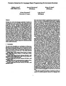
In Listing 6.2, no global of f is rebound before its application in line 3, and hence we say the closure of f is available, or shorter that f is available. As long as a closure of a function f is available, the primary environment and the closure agree on the globals of f . This relationship is called the agreement invariant. The key idea for coherence is to maintain that only functions with an available closure can be applied. The agreement invariant then justifies removing the closures. Whether a closure is available is a static property of the program which depends only on the lexical binding structure, and hence can be decided. Figure 6.1: Venn Diagram showing the Relationship of Coherence and SSA
coherent shadowing free
renamed apart (SSA)
40
Coherence
Note that every shadowing free program is coherent, because absence of shadowing ensures that no variable is rebound. For the same reason renamed apart programs are coherent. The renamed apart programs realize the SSA-condition: every variable is bound exactly once. Lexical binding ensures that every variable is defined before it can be used. Using the analogy from Section 2.4, coherence can be seen as a generalization of SSA from that abstracts from the single assignment requirement.
6.2
Coherence Conditions
In this section, we present coherence conditions which are decidable and sufficient for invariance. The inductive definition of coherence given in Figure 6.2 identifies programs which only apply functions with available closures. The coherence predicate is of the following form:
Λ | Γ ` coh s
Λ Γ s
: context (set V ) : set V : Exp
globals mapping available variables expression
The predicate Λ | Γ ` coh s should be read as Under the assumptions Λ about the globals of the available functions and the available variables Γ , s is coherent. The globals mapping Λ maps every label f to a set containing the globals of f . Every variable relevant for s must be in the set Γ of available variables. The predicate maintains the invariant that Λ only contains available functions, and the Coh-App-rule ensures only f ∈ dom Λ can be applied. Whenever a variable x is rebound, all functions that require the global x become unavailable, and are removed from Λ.
6.2.1
Rules
The rules are similar to the rules of liveness in 5.2. As in the rules for liveness, the set Γ is an over-approximation of the relevant variables. However, it is more useful to think of Γ as the set of available variables in the setting of coherence. Γ contains those variables the program may use. Λ now records the globals of each function. The globals are an over-approximation of the relevant variables of the function, and are thus similar to the live variables of the function. However, Λ has a new, second purpose: It does not contain all functions, but only those with available closures. To maintain this invariant, a function is removed if its closure is no longer available. Recall that a closure of a function f is available, as long as no global of f has been rebound.
41
Coherence
Figure 6.2: Coherence: A Sufficient Condition for Invariance
V (e) ⊆ Γ bΛcΓ \{x} | Γ ∪ {x} ` coh s Λ | Γ ` coh let x = e in s
Coh-Op
Coh-Cond
Λ | Γ ` coh s Λ | Γ ` coh t Λ | Γ ` coh if x then s else t
x∈Γ
Coh-Var
x∈Γ Λ | Γ ` coh x
Γf ⊆ Γ Coh-App
y ⊆Γ 0
Λ, f : Γf , Λ | Γ ` coh f y
Λ, f : Γf | Γ ` coh t bΛ, f : Γf cΓf | Γf ∪ x ` coh s Coh-Fun
Γf ⊆ Γ \ x
Λ | Γ ` coh fun f x = s in t
The rule Coh-Op deals with variable binding. This binding can potentially cause a closure to become unavailable. The rule uses the operation bΛcΓ := {f : Γf ∈ Λ | Γf ⊆ Γ } which restricts Λ to functions requiring at most Γ as globals. This ensure that s may only apply functions which require at most Γ \ {x} as globals. Any function requiring the variable x as global is not contained in bΛcΓ \{x} and hence unavailable in s. The rule further updates the set of available variables Γ to contain x, because x has just been bound. The rule Coh-Fun deals with function definitions. When the definition of a function f is encountered, a set Γf containing at least the globals of f is chosen and recorded in Λ. To the function body s, any variable will be available that is either a global of f (i.e. in Γf ), or a parameter of f . Since parameter binding makes any function unavailable that uses a global with the same name, Λ is restricted to Γf . For this restriction it is important that Γf does not contain parameters of f . The rules Coh-Cond, Coh-Val, Coh-App are similar to the rules for liveness from Section 5.2: The rules maintain Γ as an over-approximation of the relevant variables. In contrast to liveness, however, coherence does not need Γ to be as small as possible.
42
Coherence
6.2.2
Decidability
The rules are syntax-directed except for the non-determinism in the rule Coh-Fun. There are only finitely many choices for Γf ⊆ Γ \x, hence coherence is decidable. Theorem 10 (Coherence is Decidable) For all Λ, Γ and s, it is decidable whether Λ | Γ ` coh s. The proof of Theorem 10 is constructive and yields an extractable decision procedure.
6.3
Preservation
In this section, we show a preservation result for coherence. We introduce the notion of a coherent state and define the set of all coherent states Coh. A coherent state has two key properties: First, the program it represents is coherent, and second, all available functions satisfy the agreement invariant. We then show that Coh is closed under evaluation, i.e. that coherence and the agreement invariant are preserved under evaluation.
6.3.1
Agreement Invariant
The agreement invariant describes a correspondence between the values of variables in function closures and the primary environment. Consider the program state L, f := (Vf , x, s) | V | t If the closure of a function f is available, the closure environment Vf agrees with the primary environment V on f ’s globals Γf : Vf =Γf V . Given an environment V and contexts L and Λ, we say L, V satisfy Λ if the aforementioned condition holds for all f ∈ dom Λ. The agreement invariant is defined as follows: Definition 8 (Agreement Invariant) L, V î Λ : ⇐⇒ ∀f ∈ dom L ∩ dom Λ, Vf =Γf V
6.3.2
Context Coherence
Function application continues evaluation with the function body from the closure. Consider, for example, the evaluation
-→
L, f := (V 0 , x, s), L0 L, f := (V 0 , x, s)
43
|V x | V 0V y
|fy |s
Coherence
Figure 6.3: Context Coherence: Coherence for Contexts
Coh-Ctx-Emp
Λ ` coh L Coh-Ctx-Con
` coh
Γ ∩x= bΛ, f : Γ cΓ | Γ ∪ x ` coh s Λ, f : Γ ` coh L, f := (V , x, s)
If coherence is to be preserved, s must be coherent under suitable assumptions, too. For this purpose, we define the context coherence predicate given in Figure 6.3, which is of the following form: Λ ` coh L
Λ L
: context (set V ) : context closure
globals mapping label context
Λ ` coh L states that all function bodies in L are coherent with respect to Λ, and is defined by induction on the context according to the rules given in Figure 6.3. The rule Coh-Ctx-Con encodes the two key requirements: First, the globals of a function f must not contain a parameter of f . Second, the body of f must be coherent under the context restricted to the globals of f . Compare this to Coh-Fun in Figure 6.2, which establishes both properties. Context coherence is stable under restriction to every set of variables Γ , because restriction will only remove functions from Λ: Λ ` coh L =⇒ bΛcΓ ` coh L Context coherence is also stable under rewinding to any function f :
=⇒
6.3.3
Λ, f : Γf , Λ0 Λ, f : Γf
` coh L, f := (V , x, s), L0 ` coh L, f := (V , x, s)
Preservation Theorem
Using agreement and context coherence, we define the set of coherent states Coh as follows: Coh(Λ, Γ ) = {(L, V , s) | Λ | Γ ` coh s ∧ Λ ` coh L ∧ L, V î Λ} [ Coh = Coh(Λ, Γ ) Λ,Γ
The preservation result states that Coh is closed under evaluation. Theorem 11 Coh is -→-closed.
44
Coherence
6.4
Coherence Implies Invariance
In this section, we show that IL/F and IL/I give the same interpretation to coherent programs. This is the main result about coherence. To make our proof intention clear, we state a corollary of the main result. The following corollary states that for every label-closed, coherent program s, any functional state (including closure environments) is in bisimulation with the corresponding imperative state (without closure environments). Corollary For every well-formed program s, ◦
| Γ ` coh s =⇒ s I ∼
F
s
To obtain Corollary 1 we exhibit a state bisimulation ≈coh between coherent program states of IL/F and corresponding states of IL/I. (L, V , s) ≈coh (strip L, V 0 , s) : ⇐⇒ ∃ Λ Γ , (L, V , s) ∈ Coh(Λ, Γ ) ∧ V =Γ V 0 Theorem 12 ≈coh ⊆
I
∼
F
Corollary 1 now follows by setting L = Λ = and observing that , V î s and ` coh are vacuously true. Technically, we also need to show that any program s which satisfies | Γ ` coh s is label closed, and that evaluation of label-closed programs does not depend on the context. Theorem 12 states that coherent programs can be interpreted either as IL/F programs or as IL/I programs without changing their meaning. This is a powerful property, because Theorem 12 reduces the problem of translating between IL/I and IL/F to the problem of establishing coherence. Of course, coherence is only a sufficient criteria for invariance, but it is a decidable one. In the next chapter, coherence provides the basis for the correctness conditions of the translation between IL/I and IL/F.
45
7
Transformations
In this chapter we present two important transformations which realize the translation between IL/I and IL/F. In the previous chapter we have seen that coherent programs have the same meaning in both interpretations. To translate between the two interpretations, it hence suffices to establish coherence while preserving either the functional or the imperative semantics. We discuss establishing imperative coherence in Section 7.1. The transformation and its correctness conditions are derived from the coherence predicate. We formulate a translation predicate that relates programs to their equivalent and coherent translations. We implement the translation predicate via a correctness predicate and a compilation function in Section 7.2. The translation relies on external information, which we integrate using translation validation. Establishing imperative coherence can be seen as SSA construction with the restriction that the block structure must remain unchanged. We discuss establishing functional coherence in Section 7.3. Functional coherence can be established by α-renaming, in particular by renaming all variables apart. We relax the correctness conditions to allow α-renamings to drastically reduce the number of used variables. An α-renaming that drastically reduces the number of used variables and establishes coherence can be understood as a register assignment. The decidability result for the correctness condition is the basis for a translation validation framework for register assignment, which we explain in Section 7.3.6.
7.1
Imperative Coherence Translation
In this section, we discuss how an IL/I program can be transformed to an equivalent, coherent program. We will also refer to this transformation as establishing imperative coherence. Since a coherent program means the same in IL/I and IL/F, a transformation that establishes imperative coherence is also a transformation that translates an IL/I program to an IL/F program. We explain the translation with the help of an example. Recall that in a coherent program only functions with an available closure may be applied.
47
Transformations
IL/I programs usually rely on register reassignment quite heavily, potentially making closures unavailable. Consider the following program, which is not invariant, for example: Listing 7.1: An IL/I Program (not coherent) 1 2 3 4
let x = 7 in fun f () = x in if y then let x = 3 in f () else f ()
The closure of f becomes unavailable after the assignment to x in line 3, because x is a global of x. To ensure the closure of f remains available after the assignment, x is removed from the globals of f by making it a parameter: Listing 7.2: An IL/I Program (coherent) 1 2 3 4
let x = 7 fun f x = if y then else
in x in let x = 3 in f x f x
At all applications, the parameter itself is used as argument. The strategy to convert globals to parameters works in general, and a simple strategy to establish coherence is to make every variable in the program a parameter. For example, the following program in which all free variables have been added as parameters to every function is also coherent: Listing 7.3: An IL/I Program (coherent) 1 2 3 4
let x = 7 in fun f (x,y) = x in if y then let x = 3 in f (x,y) else f (x,y)
However, usually fewer parameters suffice. As we explained in Section 2.6, adding parameters corresponds to placing φ-functions, and minimizing the number of φ-functions is desirable for practical purposes. For this reason, we give a translation predicate to formally describe which parameters must be added to obtain a coherent program. The predicate only requires a parameter to be introduced if it is necessary to establish coherence. The translation predicate is of the following form:
Λ | Γ | Π ` s / s0
Λ Γ Π s s0
: : : : :
context (set V ) set V context (list V ) Exp Exp
globals mapping live variables additional parameters source expression target expression
The predicate Λ | Γ | Π ` s / s 0 should be read as 48
Transformations
Under the assumptions Λ about the globals of functions occurring free in s, the available variables Γ , and the additional parameters Π for functions occurring free in s, the program s 0 is a coherent program equivalent to s. Λ and Γ are used similarly to their usage in the definition of coherence. Π encodes the parameters that must be added to the functions in Λ to make the program coherent. If Λ | Γ | Π ` s / s 0 is derivable, then s 0 is obtained from s by adding the parameters as described by Π to function definitions and applications, and s 0 is coherent.
7.1.1
Rules
The rules are essentially the rules for coherence, with the twist that coherence for s 0 is ensured. The rules are defined such that s 0 is obtained from s by adding additional parameters to function definitions and applications. Figure 7.1: Translation Predicate
Trs-Op
Trs-Cond
V (e) ⊆ Γ bΛcΓ \{x} | Γ ∪ {x} | Π ` s / s 0 Λ | Γ | Π ` let x = e in s / let x = e in s 0
x∈Γ Λ | Γ | Π ` s / s0 Λ | Γ | Π ` t / t0 Λ | Γ | Π ` if x then s else t / if x then s 0 else t 0 x∈Γ Λ|Γ |Π ` x / x
Trs-Var
Γf ⊆ Γ Trs-App
yz ⊆ Γ
0
Λ, f : Γf , Λ | Γ | Π, f : z, Π0 ` f y / f yz
Λ, f : Γf | Γ | Π, f : z ` t / t 0 bΛ, f : Γf cΓf | Γf ∪ xz | Π, f : z ` s / s 0 Coh-Fun
Γf ⊆ Γ \ xz
Λ | Γ | Π ` fun f x = s in t / fun f xz = s 0 in t 0
The rules Trs-Op, Trs-Cond, and Trs-Var are analogous to Coh-Op, Coh-Cond, and Coh-Var, respectively. Each of the rules translates the program directly. The rule Trs-App is similar to Coh-App when checking for coherence of the translation f yz. The rule adds the additional parameters as arguments to the application. Otherwise the rule ensures that the globals Γf of f (which neither contain parameters nor additional parameters) are available at the application. The rule Trs-Fun deals with function 49
Transformations
definitions. The rule chooses the set of globals and a list of additional parameters z for f . Both are recorded in Λ and Π, respectively. The additional parameters z are added to the translation of the function definition. The premises are similar to Coh-Fun with xz as parameters, because coherence is ensured for the translation.
7.1.2
Decidability
We can decide whether a given set of parameters is sufficient to achieve coherence in the following sense: Theorem 13 (Correctness of Translation is Decidable) Given Λ, Γ , Π, s, s 0 , it is decidable whether Λ | Γ | Π ` s / s0 The proof of Theorem 13 is constructive and yields a decision procedure which can be used for translation validation. We explain this in detail in Section 7.2.
7.1.3
Properties of the Translation
The main property of the translation predicate is that it yields a coherent program, which we prove with the following theorem: Theorem 14 (Translation Establishes Coherence) Λ | Γ | Π ` s / s0 =⇒ Λ | Γ ` coh s 0 What remains to be shown is that the translated program is observationally equivalent to the original program. To do so, we define a relation ≈trs between source and target programs and show that the relation is a bisimulation. The programs related by ≈trs may be open, hence we need the label contexts on both sides to be correct translations of each other, too. We define the following predicate that relates two contexts L, L0 if L0 is the translation of L under the globals Λ and the additional parameters Π.
Λ | Π ` L / L0
Λ Π L L0
: : : :
L * set V L * set V context context
globals mapping additional parameters label context translated label context
The rules for context translation are given in Figure 7.2. Trs-Ctx-Con ensures that the function bodies in L and L0 are pairwise translations of each other. We can now define the relation ≈trs and show that it is a bisimulation. The relation relates states where programs and contexts are translations of 50
Transformations
Figure 7.2: Context Translation
Trs-Ctx-Emp
Trs-Ctx-Con
| ` /
Λ | Π ` L / L0 bΛ, f : Γ cΓ | Γ ∪ xz | Π, f : z ` s / s 0 Λ, f : Γ | Π, f : z ` L, f := (x, s) / L0 , f := (xz, s 0 )
each other. The variable environments are required to agree on the available variables Γ . Definition 9 (Translation Bisimulation) Translation bisimulation ≈trs is defined as (L, V , s) ≈trs (L0 , V , s 0 ) : ⇐⇒ ∃ Λ Γ Π,
Λ | Γ | Π ` s / s0 ∧ V =Γ V 0 ∧ Λ | Π ` L / L0
The simulation result is obtained with respect to the semantics of IL/I. Note that Theorem 14 ensures the translation is coherent, hence the IL/I interpretation of the original program is equivalent to the IL/F interpretation of the translation. Theorem 15 (Translation Correctness) ≈trs ⊆ ∼ As mentioned earlier, in the formal development, the translation predicate is separated into a correctness predicate and an extractable compilation function. This is described in Section 7.2.
7.2
Implementing the Translation Predicate
In section Section 7.1, we gave a translation predicate to characterize correct translations that establish imperative coherence. The translation predicate is not functional in the translation, i.e. even when fixing Λ, Γ , Π there might be several derivable translations of a program s. For example, Listing 7.2 and Listing 7.3 are both derivable translations of Listing 7.1 under Λ = Π = and Γ = {y}. In the example, the non-determinism stems from the fact that choosing both, x or x, y as additional arguments for f will yield a coherent program. In the Coq development, we realize the translation using a correctness predicate and a compilation function. As explained above, the translation predicate admits several translations, and we introduce an additional argument which replaces the translation in the correctness predicate, and fixes 51
Transformations
the additional arguments for the compilation function. The compilation function must have access to the additional parameters for functions defined inside the program. We explain how this information is encoded with the help of the following example: Listing 7.4: An IL/I program (not coherent) 1 2 3 4
fun g () = let x = y in f () in let y = 3 in g ()
Suppose that x is relevant for f . The following is a derivable translation of the above program: Listing 7.5: Translation of Listing 7.4 1 2 3 4
fun g y = let x = y in f x in let y = 3 in g y
The information that x is an additional argument for f is represented in Π, and providing Π to the compilation function would suffice to make the information available that x must be added as parameter to f . However, the information that g requires the additional parameter y, and only the additional parameter y is not recorded in Π. The information is encoded in the derivation of the translation predicate, namely as the list of additional parameters z in Trs-Fun. It is exactly this information which must be shared between the correctness predicate and the compilation function.
7.2.1
Annotations
Annotations provide a way to annotate the abstract syntax tree of the program with additional information. We explain the mechanism using Listing 7.4. The compilation function needs to know for every function definition which additional parameters are to be inserted, and for every function application which additional arguments must be inserted. In general, we want to annotate every node in the programs AST with certain information. For this purpose, we introduce a grammar that generates ASTs of the same shape as the syntax of our language, and allows information to be placed at each node. For example, Figure 7.3 shows the AST of Listing 7.4 together with the AST of the annotation providing the additional parameters and arguments required for the translation. The nodes structurally corresponding to function definitions and function applications are annotated with the list of additional parameters and arguments, in this case x and y. The annotations can be defined as shown in Figure 7.4, for example. Note that the syntax in Figure 7.4 is parametric in the type of the annotation A, and that a ranges over A by convention. A predicate s : a can be 52
Transformations
Figure 7.3: Listing 7.4 with Annotation (a) AST of Listing 7.4
(b) AST of Annotation of Listing 7.4
f un g
y
let x = y
let y = 3
f ()
g()
x
y
formulated that relates a program s and an annotation a if they are of the same shape. It is routine to show that s : a is a decidable predicate. We chose the notation for the predicate to resemble how type assignment is usually written in presentations of type systems, and in fact, type assignments can be seen as a form of annotation. Figure 7.4: Syntax of Annotations: The definition is parametric in the set of annotations A over which a ranges.
Ann 3 s, t ::= ann0 a
7.2.2
nullary annotation
| ann1 a s
unary annotation
| ann2 a s t
binary annotation
Compilation Function
We can now formulate the compilation function c which takes a program and an annotation as arguments. The definition of c is defined recursively on Exp and Ann to satisfy the following equations. We use to denote the empty list. Note that the compilation function only yields a meaningful result if s : a.
c(let x = e in s, ann1 a) = let x = e in c(s, a) c(if x then s else t, ann2 a b) = if x then c(s, a) else c(t, b) c(f y, ann0 z) = f yz c(x, ann0 ) = x c(fun f x = s in t, ann2 z a b) = fun f yz = c(s, a) in c(t, b)
53
Transformations
7.2.3
Correctness Predicate
The correctness predicate is of the form Λ | Γ | Π ` s : a where a is an annotation instead of the translation. We do not give rules for the correctness predicate, as they are very similar to the rules for the translation predicate.
7.2.4
Translation Validation: SSA Construction
Annotations provide a simple way to integrate external, unverified procedures. Suppose, for example, we want to obtain the imperative coherence translation for the label-closed program s. The external program is provided with s and computes an annotation a. The verified validator then performs the following steps: First, it ensures that s : a holds using the corresponding decision procedure. If this is not the case, compilation is aborted. Next, the validator decides if the correctness predicate | V (s) | ` s : a holds. If this is not the case, compilation is aborted. Otherwise, the compilation function c is applied and yields the transformed program. As we mentioned earlier, establishing imperative coherence is tightly related to SSA construction. We explained in Section 2.6 that adding parameters corresponds to placing φ-functions. The translation validation technique explained above can be used to translation validate an SSA construction algorithm. The construction algorithm names the places and parameters it wants to add (i.e. all positions where it wants to place a φ-function) in the form of an annotation and passes the annotation to our framework. As discussed above, the translation predicate allows a range of translations for a given program, thus giving the external program a degree of freedom which translation it wants to choose. Our verified validator ensures the annotation is satisfies the correctness predicate and translates the program accordingly. The standard SSAconstruction algorithm [20] minimizes the number of φ-functions. Our translation predicate supports minimal construction by requiring only parameters that are necessary to ensure coherence of the translation. We conjecture that as long as the block structure of the program remains unchanged, even minimal translations are derivable with our predicate, but we have no formal analysis. Traditional SSA-construction algorithms [20] reorder the block structure of the program to reduce the number of required φ-functions. We explain the issue using IL/I programs, although SSA-construction algorithms work on CFGs. Consider, for example, the program given in Figure 7.5a. Our specification is forced to introduce x as an argument to both f and g to establish coherence and yields the program shown in Figure 7.5b.
54
Transformations
Figure 7.5: An IL/I Program and Its Imperative Coherence Translation (a) Original 1 2 3 4
fun g () = x in fun f () = g () in let x = 3 in f()
(b) Translation 1 2 3 4
fun g x = x in fun f x = g x in let x = 3 in f x
The nesting structure of the original program in Figure 7.5a is flat, and this is the reason why g needs an argument. When applied to Figure 7.5a, state of the art SSA-construction algorithms will yield a CFG corresponding to the following program: 1 2 3 4 5
fun f x = fun g () = x in g () in let x = 3 in f x
The above program does not require an argument for g, and hence the corresponding CFG has less φ-functions than the CFG corresponding to our translation. If, however, the input program has already the optimal blocknesting structure, we conjecture that our translation predicate validates a minimal translation produced by state of the art construction algorithms. For example, if the following program is provided to our framework, the translation predicate admits the result of the standard SSA-construction algorithm. 1 2 3 4 5
fun f () = fun g () = x in g () in let x = 3 in f ()
We discuss an extension of our framework that would allow alterations to the block structure in Section 10.1.6.
7.3
Functional Coherence Translation
In this section, we discuss how an IL/F program can be transformed to an equivalent, coherent program. We will also refer to this translation as establishing functional coherence. As we have seen in Figure 6.1, a simple method to establish coherence for a functional program is α-renaming the program apart. The properties of α-conversion ensure semantic equivalence. This method, however, introduces a different variable for each definition. 55
Transformations
In the following we present the notion of local injectivity, which characterizes α-renamings that can drastically reduce the number of variables and at the same time establish coherence. Local injectivity will justify renaming the left program below to the right program below. As Appel [6] noted, ListListing (7.6): Program A 1 2 3
x = 7; fun f () = z in y = 5; f ()
Listing (7.7): Program B 1 2 3
x = 7; fun f () = z in x = 5; f ()
ing 7.7 can be seen as the register allocated version of Listing 7.6. We use local injectivity to provide correctness conditions for register assignment. The decidability result for local injectivity provides the basis for a translation validation framework for the register assignment phase of SSA-based register allocation [27].
7.3.1
Renaming
A renaming is a function ρ : V → V that maps variables to variables. We implicitly assume a renaming operator and write ρs for the program obtained from s by renaming all (including bound) variables according to ρ. If s is renamed apart, then for every α-equivalent program s 0 there is a renaming ρ such that s 0 can be obtained from s via renaming: ρ s = s 0 . For example, Listing 7.7 can be obtained from Listing 7.6 via ρ = {y , x}. We say ρ contracts x, y to x. Note that we define a renaming, we write the mappings that are different from the identity. If a renaming contracts too many variables (or renames free variables), the renaming will not yield an α-equivalent program. For example, renaming Listing 7.6 with {y , x, z , x} yields a semantically different program. If a program is not renamed apart, not every α-equivalent program can be obtained via a renaming, e.g. Listing 7.6 cannot be obtained from Listing 7.7 via a renaming as there is no way to assign different variables to the two binding occurrences of x.
7.3.2
Local Injectivity
We are now interested in conditions that ensure a renaming respects αconversion and yields a coherent program. Such a renaming can be used to establish functional coherence. If a renaming ρ is injective, it cannot contract variables. Such a renaming yields an α-equivalent program and preserves coherence. If the goal is to minimize the number of names, however, the injectivity condition must be relaxed. A renaming will respect α-conversion and produce a coherent
56
Transformations
program if it does not contract any two relevant variables at any point in the program. Relevance is a semantic notion, and we resort to a construction similar to liveness from Chapter 5 to over-approximate the set of relevant variables. We build this over-approximation into our notion of local injectivity, together with the appropriate injectivity conditions. Local injectivity is defined as a predicate of the following form:
Λ | Γ ` inj ρ s
Λ Γ ρ s
: : : :
L * set V set V V →V Exp
globals mapping live variables renaming expression
The predicate Λ | Γ ` inj ρ s should be read as follows: The renaming ρ is locally injective for the program s given the liveness assumptions Λ and Γ .
7.3.3
Rules
The rules defining the predicate are given in Figure 7.6. We use the following notation for injectivity: f � Γ : ⇐⇒ ∀x y ∈ Γ , f x = f y =⇒ x = y The rules are extensions of the rules for liveness from Section 5.2 with additional injectivity requirements. Every rule requires ρ � Γ , ensuring Λ | Γ ` inj ρ s =⇒ ρ � Γ This means that the renaming must be injective on every set of live variables occurring in the derivation. The rule Inj-Op deals with variable definitions. The renaming must be injective on the set containing x and the live variables of the continuation s. Example 9 below shows why including x is critical even if x is never used in s. The rules Inj-Cond, Inj-Val and Inj-App correspond to the liveness rules from Section 5.2, each with the additional injectivity requirement. Inj-Fun deals with function definitions. The premises are, again, the same as for Live-Fun, with the addition of injectivity requirements. The important requirement here is that ρ is injective on the set containing both the variables live in the function body and the parameters. We explain the reason in Example 10. Example 9 The rule Inj-Op requires ρ � Γ 0 ∪ {x}. To see why this is important, consider the following program: 1
let x = z in y
Obviously x is not relevant for y. If we would not require ρ � Γ 0 ∪ {x}, then ρ = {x , y} would be locally injective for the above program, yielding 57
Transformations
1
let y = z in y
which clearly is a different program. Example 10 The rule Inj-Fun requires ρ � Γf ∪ x. To see why this is important, consider the following program: 1 2
fun f x = y in f z
Obviously, x is not relevant for f . If we would not require ρ � Γf ∪ x, then ρ = {x , y} would be locally injective for the above program, yielding 1 2
fun f y = y in f z
which is clearly a different program.
Figure 7.6: Local Injectivity
ρ�Γ ρ � Γ 0 ∪ {x}
V (e) ⊆ Γ Γ \ {x} ⊆ Γ 0
Inj-Op
Λ | Γ 0 ` inj ρ s
Λ | Γ ` inj ρ let x = e in s Λ | Γ 0 ` inj ρ s {x} ∪ Γ 0 ∪ Γ 00 ⊆ Γ
Inj-Cond
Λ | Γ ` inj ρ if x then s else t
Inj-Val
Inj-App
Γ0 ⊆ Γ Γf ⊆ Γ \ x Inj-Fun
Λ | Γ 00 ` inj ρ t
ρ�Γ
x∈Γ ρ�Γ Λ | Γ ` inj ρ x
y ∪ Γf ⊆ Γ
ρ�Γ
0
Λ, f : Γf , Λ | Γ ` inj ρ f y ρ�Γ ρ � Γf ∪ x
Λ, f : Γf | Γf ∪ x ` inj ρ s Λ, f : Γf | Γ 0 ` inj ρ t
Λ | Γ ` inj ρ fun f x = s in t
58
Transformations
7.3.4
Decidability
Local injectivity is decidable as there is only a finite number of choices for Γf in Inj-Fun. The following lemma yields a decision procedure. Theorem 16 (Local Injectivity is Decidable) For all Λ, Γ , ρ, and s, Λ | Γ ` inj ρ s is decidable.
7.3.5
Properties of Locally Injective Renamings
The two key properties of locally injective renamings are that they respect α-conversion and establish coherence. We first prove that local injectivity is sufficient to guarantee coherence of the renamed program. To state the result some definitions are required. VB (s) denotes the set of variables that occurs in a binding position in s. The following notation for a context Λ and a set U expresses that every set in Λ is bounded by U : Λ ⊆ U : ⇐⇒ ∀f ∈ dom Λ, Λ f ⊆ U We are now ready to state the theorem: Theorem 17 For all well-formed, renamed-apart programs s and sets of variables U such that VB (s) ∩ U = , Λ ⊆ U =⇒ Λ | Γ ` inj ρ s =⇒ ρ bΛcΓ | ρ Γ ` coh ρ s The theorem requires a renamed-apart program s, and that none of the globals recorded in Λ occur in binding positions in s. This condition holds without further ado when descending into a renamed apart program s. The conclusion of the theorem states that the renamed program ρs is coherent under the available variables ρ Γ , i.e. the point-wise renaming of Γ according to ρ. The assumptions in the coherence predicate are ρbΛcΓ . bΛcΓ restricts Λ to functions with available closures, see Section 6.1. This is necessary because renaming may have caused some closures to become unavailable, as we explain in Example 11. The restricted context is then translated by ρ in the obvious, point-wise manner. Example 11 Consider the following program, for which ρ = {y , x} is locally injective. 1 2 3 4
let x = 7 in fun f () = x in let y = 5 in y
Renaming with ρ yields the following program: 1 2 3 4
let x = 7 in fun f () = x in let x = 5 in x
59
Transformations
The renaming made f unavailable in line 4 of the latter program, and this is the reason why the restriction operator appears in the conclusion of Theorem 17. The proof of Theorem 17 requires a monotonicity property of coherence which is interesting in its own right. To state monotonicity, we require the notion of approximation on partial functions (and, by abuse of notation, on contexts): A function f approximates g if f agrees with g on dom f : f � g : ⇐⇒ ∀x ∈ dom f , f x = g x Coherence is monotonic in in the following way: The set of available variables may always be increased. Additional functions may always be added to the set of available functions Λ. The globals of the functions in Λ, however, must not be changed. In fact, any set of globals in Λ can be replaced by a smaller set, but we do not prove this property. Lemma 7 (Monotonicity of Coherence) For all programs s, contexts Λ, Λ0 and sets of variables Γ , Γ 0 Λ | Γ ` coh s =⇒ Λ � Λ0 =⇒ Γ ⊆ Γ 0 =⇒ Λ0 | Γ 0 ` coh s The second property of locally injective renamings is that they respect α-conversion. This property is important, because it shows that locally injective renamings preserve the semantics of the program. Theorem 18 For all well-formed and renamed-apart programs s, Λ | Γ ` inj ρ s =⇒ ρ s ∼α s
7.3.6
Translation Validation: Register Assignment
The results from this section can be combined to obtain a translation validation framework for register assignment. The approach fits best with SSA-based register allocation approaches such as [27]. Register assignment can be seen as renaming with a locally injective renaming. A locally injective renaming is an α-renaming that establishes coherence. In this sense, register assignment is a transformation that accomplishes the translation from an IL/I program to an IL/F program: Since the renamed program is coherent it already is an IL/I program. Determining the register assignment is usually done heuristically in production compilers. We think that heuristic parts of a compiler should be exchangeable without redoing correctness proofs. This provides flexibility to compiler implementers and researchers when integrating or developing new algorithms. The result of the heuristic is hence translation validated. Our framework renames the program apart and passes it to an external algorithm that computes a register assignment. The external algorithm can 60
Transformations
pass all required information to our framework in the form of a renaming ρ. Theorem 16 provides the procedure for deciding whether ρ is locally injective. Correctness follows from two facts. First, the renamed program is an α-equivalent program by Theorem 18, hence semantically equivalent. Second, the renamed program is coherent by Theorem 17, an hence can also be viewed as an IL/I program. In the compiler construction setting, register assignment is tightly connected to a live variables analysis. This connection becomes very explicit in our correctness analysis. The rules in Figure 7.6 are essentially the rules for liveness from Figure 5.1, extended with appropriate injectivity conditions. Despite the fact that liveness is an inherently imperative notion, the register assignment transformation is verified with respect to the functional semantics. The connection to the imperative semantics is only through coherence. This means that in our framework, register allocation is a functional transformation, not an imperative one. Section 5.3 explains that true liveness is a sharper notion of liveness. Nevertheless, true liveness does not allow better register allocations than liveness alone. The additional injectivity condition requiring ρ � Γ ∪ x in the rule Inj-Fun annihilates the advantage. The condition requires the renaming to be injective on all parameters, even if true liveness asserts that certain parameters are not live. This is important to obtain an α-equivalent program for a reason discussed in Example 9. However, true liveness can be used to perform a dead variable elimination before register assignment. In this way, a more efficient register assignment may be possible.
61
8
Formal Development
In this section, we give an overview of the development. We highlight aspects that worked well and report the size of the different modules. The source code of the formal development is available at http://www.ps.uni-saarland.de/~sdschn/master Some of parts of the development infrastructure are taken from a recent research immersion lab [58].
8.1
Infrastructure
We use the extractable set library by Lescuyer [42]. Building on it, we formalize basic notions such as injectivity and agreement of functions, together with some decidability results in the module Constr. To obtain the decision procedures described in the previous chapters, decidability results are paired with extractable decision procedures. Many definitions in this part of the development are parametrized by the equivalences on all involved types. This requires setoid rewriting [60] and increases proof detail. The module Infra in the development provides infrastructure such as an option monad [3], basic facts about lists, and a type class for decidable propositions. Both modules are rather extensive, and we feel most of the theorems should be provided by a generic library. Figure 8.1: Infrastructure: Lines of Code in Specification, Proof and Comments. Number of Lemmas and Definitions. File Infra Constr P
8.1.1
Spec 980 1213 2193
Proof 580 907 1487
Comments 111 239 350
Lemmas 160 225 385
Definitions 38 14 52
Decidable Propositions
We use a type class for decidable propositions. The type class initially developed in a recent research immersion lab [58] by Steven Schäfer. The type 63
Formal Development
class allows us to apply compute_prop to any proposition, and have Coq infer the decision procedure if it is available as instance of Computable. 1
Class Decidable (P : Prop) := decide : { P } + { ∼P }.
As part of the infrastructure, we have to prove some simple statements about decidability. Suppose we want to show that a predicate P : X → Prop is decidable. If the decision procedure is simple, it can directly be given as a function of type ∀(x : X), {P x} + {¬P x}. If the decision procedure is more complex, in particular, if the usually inductive correctness argument requires a stronger invariant than {P x} + {¬P x}, then the following strategy worked well for us. We first define a decision procedure dec 0 : X → bool which decides the proposition and is suitable for extraction. We then relate the decision procedure to P by proving ∀(x : X), dec 0 x = true ⇐⇒ P x The proof of this theorem may involve a strengthened induction hypothesis. Finally, we use dec 0 to define dec : ∀(x : X), {P x} + {¬P x} by starting with a case distinction on dec x. Using an inline hint, extraction of dec will then reduce to dec 0 .
8.2
Formalizing IL
We formalize IL as a language with explicit names for variables, and a DeBruijn-style discipline for labels. The main part of the development factors out the language of simple expressions. The idea is that the simple expressions can be instantiated with different expression languages. An instruction set architecture (ISA) can then be integrated as a special expression language. In our development, we fixed the expression language, but use only basic properties of it. We expect our development to scale without effort to any pure expression language. Figure 8.2: Expression Language: Lines of Code in Specification, Proof and Comments. Number of Lemmas and Definitions. File Val.v Exp.v P
Spec 24 74 98
Proof 0 78 78
Comments 6 9 15
Lemmas 3 19 22
Definitions 5 9 14
Figure 8.3 gives an overview of the files used for the formalization of the language IL and the dual semantics. The file ILN.v contains proofs that our context-based semantics coincides with a standard semantics. The file Sim.v contains the formalization of deterministic reduction systems and the proof that the instantiation for IL/F yields a congruence. 64
Formal Development
Figure 8.3: IL: Lines of Code in Specification, Proof and Comments. Number of Lemmas and Definitions. File IL.v Var.v Env.v ILN.v Sim.v P
8.3
Spec 233 70 4 186 168 661
Proof 37 17 0 147 407 608
Comments 19 14 8 7 25 73
Lemmas 8 13 0 12 39 72
Definitions 17 12 2 20 8 59
Coherence
The main theorems from Chapter 6 are developed in the files shown in Figure 8.4. The definition of coherence is in Coherence.v together with its simulation result. The file ILIToILF.v contains the formalization of the imperative coherence translation from Section 7.1. α-equivalence is developed in the file Alpha.v, and theorems about renaming are in Rename.v. The theorems about functional coherence construction from Section 7.3 are in RegAlloc.v. The translation validators described in Section 7.2 and Section 7.3.6 are in Compiler.v. ParallelMove.v contains a translation validation algorithm for parallel move lowering and was developed by Tobias Tebbi in a previous research immersion lab [58]. Figure 8.4: Coherence: Lines of Code in Specification, Proof and Comments. Number of Lemmas and Definitions. File ILRaise.v ILTypes.v Compiler.v ParamsMatch.v Alpha.v Liveness.v ILIToILF.v EnvTy.v Coherence.v ParallelMove.v Fresh.v RenameApart.v RegAlloc.v P
Spec 24 168 44 109 93 201 84 51 287 132 35 65 109 1402
Proof 27 123 35 38 177 276 117 48 373 88 70 225 171 1768
Comments 7 17 3 22 3 15 13 9 21 6 3 22 26 167
65
Lemmas 5 23 2 12 13 20 8 19 35 8 8 10 14 177
Definitions 0 18 2 8 4 16 3 5 14 8 3 1 7 89
9
Related Work
9.1
Static Single Assignment Form
Static single assignment form is the culmination point of a line of research in data-flow analysis. The key contributions seem to be by Rosen, Wegman, and Zadeck [55] and Alpern, Wegman, and Zadeck [5]. The standard reference for SSA-form seems to be Cytron et al. [20], which contains an efficient SSA-construction algorithm. An alternative construction algorithm is given by Braun et al. [13]. SSA form was originally invented to lower the complexity of reaching definition analysis [1]: In an imperative program, the reaching definition relation is potentially quadratic in the program size (assuming only one register, every definition could reach every use). If every variable has at most one definition, the relation is trivially linear in the program size. Zadeck [64] gave a talk about the origin of SSA form. The correspondence between SSA form and functional programming is due to Appel [7] and Kelsey [36]. Later Chakravarty, Keller, and Zadarnowski [15] investigated SSA optimizations on functional programs. Typical SSA optimizations include global value numbering (GVN) [55], sparse conditional constant propagation [63], and partial redundancy elimination [62].
9.2
SSA and Functional Programming
Continuation Passing Style (CPS) has played a fundamental role for both practical compilation and programming languages research in general. We refer the reader to Reynolds [53] who accounts for the numerous discoveries of continuations in literature. The first-order restriction of our language does not allow CPS-style programs. CPS has been used in the compilation of functional languages [6]. The transformation to CPS produces a large number of λ-expressions. Danvy and Filinski [22] single out administrative λ-expressions and devise a restricted form of β-reduction to eliminate them. Sabry and Felleisen [56] prove the resulting reduction system confluent and terminating, a result which gives rise to administrative normal form (ANF). Flanagan et al. [24]
67
Related Work
show that ANF form can be constructed directly from a functional source language without applying a CPS transformation first. Our intermediate language is in administrative normal form, and in particular, IL/F is a sub-language of the ANF language presented in Chakravarty, Keller, and Zadarnowski [15]. Kelsey [36] seems to be the first to translate SSA programs to CPS programs, although Kelsey states the correspondence had been noted by others [6, 47]. Chakravarty, Keller, and Zadarnowski [15] translates SSA to ANF and reformulate the SSA-based sparse conditional constant propagation optimization [63] on their functional ANF language.
9.3
Control Flow and Recursive Functions
The control-flow graph (CFG) as a means to analyze the structure of imperative programs is due to Allen [4]. Prosser [52] used Boolean connectivity matrices to represent control flow before Allan. Allen [4] also classified flow graphs as either reducible or irreducible. Hecht and Ullman [30] found a second characterization of reducibility and showed that structured control flow always yields a reducible control-flow graph, while unstructured control flow may yield an irreducible control-flow graph. Hecht and Ullman [29] compiled a list of alternative characterizations of reducibility. From the translations given by Kelsey [36] and Chakravarty, Keller, and Zadarnowski [15], it is clear that unstructured control flow can be expressed via mutually recursive functions. It seems to be generally acknowledged that reducible control flow can be directly represented without mutual recursion. However, we have not found a reference that definitely asserts this claim. The origins of analyses on CFGs such as reaching definitions and live variables seems to be difficult to attribute. Hecht [28] wrote in 1977 that the definitions appear in a large number of papers. According to Seidl, Wilhelm, and Hack [57], the notion of true liveness originates from Giegerich, Möncke, and Wilhelm [25].
9.4
Verified Compilers for C-like languages
Two major verification projects for compilers of C-like languages exist. CompCert [3] is a verified compiler for a realistic subset of the C language. Even non-optimizing translation passes were difficult to verify [40]. For this reason, CompCert follows a conservative design without SSA form, which includes constant propagation, local common sub-expression elimination, and register allocation as central optimizations. Leroy [38] notes that SSA form was originally not integrated into CompCert because it is not obvious to formalize. Advanced, SSA-based optimizations for CompCert are 68
Related Work
available via the CompCertSSA project [10, 26], but they have not been reintegrated into main-line CompCert. A formalization of the semantics of the C language can be found in Norrish [46]. The VeLLVM Project [67] is an ongoing effort to verify the production compiler LLVM [19] including its advanced, production-grade optimizations. The VeLLVM project has recently completed all steps [66, 68, 65] to verify the standard SSA-construction algorithm [20]. The intermediate language of LLVM is an imperative intermediate language with φ-functions to enable SSA form [66].
9.5
Related Work for Bisimulations
Alternative characterizations of program equivalence for the purpose of proof are standard in the literature: Logical relations [49] and bisimulations are the most prominent examples. Pitts [50] gives an introduction how to show that the bisimulation characterization coincides with contextual equivalence based on Howe’s method [31, 32] for the simply-typed λcalculus. Howe’s method is a robust proof method developed for higherorder functional languages. Recently, Hur et al. [33] have presented a hybrid approach of bisimulations and logical relations. Bisimulations are used heavily for model checking [8]. Our first-order setting simplifies proving the congruence property of our simulation and none of the advanced methods are required. In fact our bisimulation does not even have to be applicative in Howe’s sense, as equality only arises on base types. Simulations have been used for proving semantic preservation in the CompCert project [38]. There are two main differences: On one hand, we prove that our bisimulation characterization is a congruence (in fact it coincides with contextual equivalence). On the other hand, CompCert has richer observable behavior, as it includes the ordered list of externally visible events the program produces. Our Theorem 1 shows that our bisimulation fully characterizes observational equivalence. CompCert only shows the equivalent of the right-to-left direction of Theorem 1.
9.6
Research Compilers with Functional Intermediate Languages
Many recent research compilers already employ essentially functional intermediate languages. Compilers often strive to normalize the source program as aggressively as possible. Functional languages aid this process because syntactically equivalent fragments usually have the same meaning. Johnson and Mycroft [34] use this idea to do code minimization on a program
69
Related Work
representation they call value state dependence graph, which is essentially a functional intermediate language. Tate et al. [61] introduce the program expression graph (PEG), an aggressively normalizing, graph-based program representation that can accommodate alternative representations for every node. Optimization is then performed by selecting the most beneficial representative for each node. The lazy functional semantics of PEGs is especially beneficial for the justification of aggressive loop optimizations that would be hard to argue correct using an imperative semantics. libFirm [2] is a research compiler that uses an essentially functional intermediate representation and exploits properties for optimizations. An important idea in compiler construction are sea-of-nodes intermediate representations put forward by Click and Cooper [16] and Click and Paleczny [17]. The key idea of the sea-of-nodes approach is to represent the program as a graph with a fully compositional notion of program equivalence. Many optimizations are characterized by equivalence respecting rewriting operations, hence to establish correctness for an optimizations, it suffices to argue locally that the transformation is semantics preserving. The research compilers mentioned before [34, 61, 2], and the productiongrade Java HotSpot VM [48] build to different degrees on the sea-of-nodes idea.
9.7
Languages with Dual Interpretation
Kelsey and Hudak [37] constructed a compiler with a single intermediate language that consists of both, functional and imperative features. To produce an assembly program, the intermediate language is transformed to a subset of the language that corresponds to assembly, and this subset has a dual semantics, in particular, variables can be seen as either functional variables or as registers. We take up this idea, and give a mechanized treatment of the approach. Beringer, MacKenzie, and Stark [12] used a language with a functional and imperative interpretation for proof carrying code. They give a sufficient condition for the two semantics to coincide which they call Grail normal form. Their notion requires functions to not use the closure at all, i.e. a function must only depend on its parameters. This makes the notion significantly weaker than ours. The requirement that a function must only depend on its parameters corresponds to maximal insertion of φ-functions, which is not suitable for SSA construction. The relation of register assignment to α-equivalence is not explored.
70
Related Work
9.8
Translation Validation
An important concept in compiler verification is translation validation [51]. In translation validation, not the translation itself is verified, but a (usually simpler) validator that decides after the fact whether the translation was sound. An explanation of the significance of translation validation for compiler verification has been given by Leroy [40]. Our approach is based on translation validation: Our correctness criteria rely on external information, which we validate using a verified validator to ensure correctness. For example, in Section 7.3.6, we gave a translation realizing register assignment. This translation depended on a renaming which represented the register assignment. The renaming must be locally injective for the register allocation to be correct, and we use translation validation to ensure that the renaming is locally injective.
9.9
Register Transfer Languages
A definition of the term register transfer (RT) can be found in Bell and Newell [11], which use register transfers as a means to describe hardware components more abstractly. Davidson and Fraser [23] use register transfers as unified way to ascribe semantics to assembly instructions from different instruction sets. More recently, the term register transfer language (RTL) seems to be used for a language where (a) there are global names for each address (b) addresses cannot be generated programmatically (c) addresses hold a scalar value (not a compound value) . The languages may have other features, like function calls and allocatable memory, as well. Examples for the use of the term RTL in this way are Leroy [39] and the GCC project [18].
9.10
Register Allocation
SSA-based register allocation [27] consists of three phases. The first phase is called spilling and ensures that at no point more than a fixed number of registers are required by inserting loads and stores to the memory. The second phase is register assignment. Register assignment assigns each pseudoregister a machine register. After the spilling phase this is always possible. The third phase is called coalescing. In an SSA-based setting, φ-nodes, or in our case, function arguments have to be implemented via parallel assignments. Coalescing tries to reassign registers to minimize the number of required assignments. Our framework supports register assignment. An external program could pass the result of register allocation including coalescing as renaming, hence the only missing phase is spilling.
71
10
Conclusion
An intermediate language for the back-end of a compiler was presented. The dual interpretation of the intermediate language makes it fit for two purposes: The imperative interpretation provides a low-level language useful for the later stages of code generation towards a (virtual) machine. The language has enough structure to represent all important back-end compilation decisions, such as code scheduling [1] and register allocation. The functional interpretation is a first-order language in administrative normal form with a tail-call restriction. Program equivalence on IL/F is fully compositional. The language can serve as an entry point for the translation to a more expressive functional intermediate language. Integration is simple if the richer language contains IL/F as a fragment. The richer language could, for example, include higher-order features or lift the tail-call restriction to allow inter-procedural optimizations. The central notion in our analysis of IL/I and IL/F is coherence. Coherence identifies programs that mean the same in both interpretations, i.e. programs that can be interpreted as either low-level programs working on an imperative machine, or as programs in a pure, first-order functional language. Coherence formed the basis for the correctness criteria of the translation between the two interpretations. Verified translation validators were implemented for both translations. The approach with a dual interpretation has proved effective for the translation between imperative and functional languages. The approach also lead to the notion of coherence, which provides a novel, more general characterization of the SSA-invariant. From a practical perspective, the translations between the two interpretations can be understood as well known transformations from compiler construction. Making an IL/I program coherent can be seen as a form of SSA construction where the block structure must remain unchanged. The transformation that makes IL/F programs coherent realizes register assignment. Our proofs show that the translation is minimally invasive in the sense that even errors are preserved. In our setup, SSA construction and register assignment are the gateway transformations between the functional and the imperative world. Their correctness criteria were derived from first principles. At the moment SSA construction is not allowed to alter the block structure of the source program. On the positive side, the graph-theoretic 73
Conclusion
concept of dominance usually used in SSA literature [20] was not required. The formalization of the intermediate language together with the correctness proofs was done using the proof assistant Coq and is completely constructive: No axioms were used. All transformations and translation validators are extractable to executable code. The formal development is available at http://www.ps.uni-saarland.de/~sdschn/master.
10.1
Limitations and Future Work
The language IL presented in this thesis is designed in such a way that its two interpretations IL/I and IL/F exactly correspond to each other. This idealization results in a loss of expressivity. IL is missing features that are required for realistic compilation. This section discusses limitations and directions for future work.
10.1.1
Observable Events
Deterministic reduction systems were used to obtain a proof technique for program equivalence. Deterministic reduction systems relied on a notion of observations, however, we only allowed observations to be made about normal programs, i.e. programs that do not reduce any more. This restricts the equivalence to be sensitive to error and result values, but explicitly excludes observations occurring during reduction, such as external events like system calls, for example. In particular, all diverging programs are regarded as equivalent. Future work is to integrate observable events during reduction into IL, for example, to accommodate system calls. If DRS would allow observations about intermediate states, DRS could potentially account for events. The effects of introducing events on contextual equivalence would have to be investigated.
10.1.2
Higher-Order Coherence
A possible extension is to include higher-order functions and try to recover a notion of coherence. Since in the presence of higher-order functions, sophisticated control flow structure can be encoded in CPS-style, it seems likely that not all programs can be made coherent. This means that on the imperative side, a mechanism that allows to implement the closures of selected functions must be present. An alternative would be to forbid control flow structures that cannot be realized without closures via appropriate conditions. However, it is not clear what such conditions would be, and whether the resulting fragment is practically useful. Introducing higherorder functions would require changes in the setup of the language. The
74
Conclusion
distinction between variables and labels would have to be removed.
10.1.3
Function Calls
Another possible extension is a syntactic form let x = f (x) in s which lifts the tail-call restriction. A stack discipline must then be added to both IL/F and IL/I to account for function application. The immediate benefit is that inter-procedural optimizations are enabled instantly. However, the notion of coherence must be adapted to the new language feature. It is also unclear whether IL/I with a stack discipline makes sense as a machine model.
10.1.4
Dynamic Memory Allocation
A key feature left out in our treatment is dynamically allocatable memory. At the moment, IL cannot represent programs that use dynamic memory allocation. Jung [35] explored an extension of IL/F to treat dynamic memory allocation.
10.1.5
Register Allocation
To complete verification of a register allocator, the spilling phase needs to be verified. The open question is how a translation validation based implementation of spilling would have to be designed. The key ingredient is a generic correctness criterion that allows the unverified spiller maximal flexibility. This extension can only be effectively verified in the presence of a robust and efficient framework for allocatable memory.
10.1.6
Irreducible Control Flow via Mutual Recursion
An interesting extension of the language are mutually recursive definitions. For this purpose the syntax would have to allow function definitions of the form fun f x = s in t where each fi can call any fj . This new language can directly represent irreducible control flow, and does not have to encode it. This is important from a compiler construction perspective because translating irreducible control flow to reducible control flow may increase the size of the program exponentially [14]. The extended language would allow the imperative coherence transformation to alter the block structure of the IL/I program, as discussed in Section 7.2.4. This could lead to a formal investigation of more restricted versions of SSA form that limit the number of φ-functions, such as minimal SSA form [21, 13].
75
Conclusion
It could be interesting to give a formal account of reducible control flow and show that it can be expressed without mutual recursion and without exponential increase of the program size.
10.1.7
Liveness
Liveness conditions are a reoccurring theme in the transformations presented in this thesis. From the Coq engineering standpoint, it would be interesting to find a efficient way to extract the liveness conditions from the correctness conditions for the transformations. Such a division could improve modularity of the development.
10.1.8
Optimizations
IL is a step towards the integration of advanced optimizations. To evaluate our initial assumption that functional intermediate languages are well suited for compiler optimizations, some exemplary optimizations would have to be implemented. The next step would be to define a suitable extension of IL/F to at least validate the β-rule. However, it is not clear how to set up correctness proofs for optimizations most flexibly. Ideally, the correctness arguments should be as generic as possible to ensure they are tolerant against minor modifications in the optimizations. In the best-case scenario, a generic correctness argument can be used to justify several optimizations.
76
Bibliography
[1]
Alfred V. Aho, Monica S. Lam, Ravi Sethi, and Jeffrey D. Ullman. Compilers: Principles, Techniques, and Tools (2nd Edition). Boston, MA, USA: AddisonWesley Longman Publishing Co., Inc., 2006 (cit. on pp. 12, 13, 21, 32, 67, 73).
[2]
Gerhard Goos et al. libFirm. 2012. url: http://pp.ipd.kit.edu/firm/ (cit. on pp. 1, 70).
[3]
Xavier Leroy et al. CompCert. 2012. url: http://compcert.inria.fr/ (cit. on pp. 63, 68).
[4]
Frances E. Allen. “Control flow analysis”. In: SIGPLAN Notices 5.7 (July 1970), pp. 1–19 (cit. on pp. 5, 68).
[5]
Bowen Alpern, Mark N. Wegman, and F. Kenneth Zadeck. “Detecting Equality of Variables in Programs”. In: Conference Record of the Fifteenth Annual ACM Symposium on Principles of Programming Languages. San Diego, CA, USA, Jan. 10–13, 1988, pp. 1–11 (cit. on pp. 1, 7, 67).
[6]
Andrew W. Appel. Compiling with Continuations. Cambridge, England: Cambridge University Press, 1992 (cit. on pp. 11, 56, 67, 68).
[7]
Andrew W. Appel. “SSA is Functional Programming”. In: SIGPLAN Notices 33.4 (Apr. 1998), pp. 17–20 (cit. on pp. 1, 8, 9, 67).
[8]
Christel Baier and Joost-Pieter Katoen. Principles of Model Checking. Representation and Mind Series. Cambridge, MA, USA: The MIT Press, 2008 (cit. on pp. 25, 69).
[9]
H. P. Barendregt. The Lambda Calculus Its Syntax and Semantics. Revised. Vol. 103. Studies in Logic and the Foundations of Mathematics. Amsterdam, The Netherlands: North Holland, 1984 (cit. on p. 12).
[10]
Gilles Barthe, Delphine Demange, and David Pichardie. “A Formally Verified SSA-Based Middle-End - Static Single Assignment Meets CompCert”. In: Programming Languages and Systems - 21st European Symposium on Programming. Vol. 7211. Lecture Notes in Computer Science. Tallinn, Estonia, Mar. 24–Apr. 1, 2012, pp. 47–66 (cit. on pp. 1, 69).
[11]
C. Gordon Bell and Allen Newell. Computer Structures: Readings and Examples. McGraw-Hill Computer Science Series. New York, NY, USA: McGraw-Hill, 1971 (cit. on p. 71).
77
Bibliography
[12]
Lennart Beringer, Kenneth MacKenzie, and Ian Stark. “Grail: a Functional Form for Imperative Mobile Code”. In: Electr. Notes Theor. Comput. Sci. 85.1 (2003), pp. 3–23 (cit. on pp. 1, 10, 70).
[13]
Matthias Braun, Sebastian Buchwald, Sebastian Hack, Roland Leißa, Christoph Mallon, and Andreas Zwinkau. “Simple and Efficient Construction of Static Single Assignment Form”. In: Compiler Construction - 22nd International Conference. Proceedings. Vol. 7791. Lecture Notes in Computer Science. Rome, Italy, Mar. 16–24, 2013, pp. 102–122 (cit. on pp. 7, 67, 75).
[14]
Larry Carter, Jeanne Ferrante, and Clark Thomborson. “Folklore confirmed: reducible flow graphs are exponentially larger”. In: Conference Record of POPL 2003: The 30th SIGPLAN-SIGACT Symposium on Principles of Programming Languages. New Orleans, LA, USA, Jan. 15–17, 2003, pp. 106–114 (cit. on p. 75).
[15]
Manuel M. T. Chakravarty, Gabriele Keller, and Patryk Zadarnowski. “A Functional Perspective on SSA Optimisation Algorithms”. In: Electr. Notes Theor. Comput. Sci. 82.2 (2003), pp. 347–361 (cit. on pp. 1, 9, 12, 67, 68).
[16]
Cliff Click and Keith D. Cooper. “Combining Analyses, Combining Optimizations”. In: ACM Trans. Program. Lang. Syst. 17.2 (1995), pp. 181–196 (cit. on p. 70).
[17]
Cliff Click and Michael Paleczny. “A Simple Graph-Based Intermediate Representation”. In: Papers from the 1995 ACM SIGPLAN Workshop on Intermediate Representations. San Francisco, CA, USA, Jan. 22, 1995, pp. 35–49 (cit. on p. 70).
[18]
GCC Contributors. GCC Documentation. 2013. url: http://gcc.gnu.org/ onlinedocs/ (cit. on p. 71).
[19]
LLVM Contributors. LLVM. 2012. url: http://llvm.org/ (cit. on p. 69).
[20]
Ron Cytron, Jeanne Ferrante, Barry K. Rosen, Mark N. Wegman, and F. Kenneth Zadeck. “An Efficient Method of Computing Static Single Assignment Form”. In: Conference Record of the Sixteenth Annual ACM Symposium on Principles of Programming Languages. Austin, Texas, USA, Jan. 11–13, 1989, pp. 25–35 (cit. on pp. 11, 54, 67, 69, 74).
[21]
Ron Cytron, Jeanne Ferrante, Barry K. Rosen, Mark N. Wegman, and F. Kenneth Zadeck. “Efficiently computing static single assignment form and the control dependence graph”. In: TOPLAS 13.4 (Oct. 1991), pp. 451–490 (cit. on pp. 7, 75).
[22]
Olivier Danvy and Andrzej Filinski. “Representing Control: A Study of the CPS Transformation”. In: Mathematical Structures in Computer Science 2.4 (1992), pp. 361–391 (cit. on p. 67).
[23]
Jack W. Davidson and Christopher W. Fraser. “The Design and Application of a Retargetable Peephole Optimizer”. In: ACM Trans. Program. Lang. Syst. 2.2 (1980), pp. 191–202 (cit. on p. 71).
[24]
Cormac Flanagan, Amr Sabry, Bruce F. Duba, and Matthias Felleisen. “The essence of compiling with continuations (with retrospective)”. In: 20 Years of the ACM SIGPLAN Conference on Programming Language Design and Implementation 1979-1999, A Selection. 2004, pp. 502–514 (cit. on pp. 9, 67).
78
Bibliography
[25]
Robert Giegerich, Ulrich Möncke, and Reinhard Wilhelm. “Invariance of Approximate Semantics with Respect to Program Transformations”. In: GI 11. Jahrestagung in Verbindung mit Third Conference of the European Cooperation in Informatics (ECI). Proceedings. Vol. 50. Informatik-Fachberichte. München, Germany, Oct. 20–23, 1981, pp. 1–10 (cit. on pp. 35, 68).
[26]
Delphine Demange Gilles Barthe and David Pichardie. CompCertSSA. 2012. url: http://compcertssa.gforge.inria.fr/ (cit. on p. 69).
[27]
Sebastian Hack, Daniel Grund, and Gerhard Goos. “Register Allocation for Programs in SSA-Form”. In: Compiler Construction, 15th International Conference. Proceedings. Vol. 3923. Lecture Notes in Computer Science. Vienna, Austria, Mar. 30–31, 2006, pp. 247–262 (cit. on pp. 2, 56, 60, 71).
[28]
Matthew S. Hecht. Flow Analysis of Computer Programs. New York, NY, USA: Elsevier North-Holland, Inc., 1977 (cit. on pp. 21, 32, 68).
[29]
Matthew S. Hecht and Jeffrey D. Ullman. “Characterizations of Reducible Flow Graphs”. In: J. ACM 21.3 (1974), pp. 367–375 (cit. on p. 68).
[30]
Matthew S. Hecht and Jeffrey D. Ullman. “Flow Graph Reducibility”. In: Proceedings of the 4th Annual ACM Symposium on Theory of Computing. Denver, CO, USA, May 1–3, 1972, pp. 238–250 (cit. on pp. 6, 68).
[31]
Douglas J. Howe. “Equality In Lazy Computation Systems”. In: Proceedings of the Fourth Annual Symposium on Logic in Computer Science. Pacific Grove, CA, USA, June 5–8, 1989, pp. 198–203 (cit. on p. 69).
[32]
Douglas J. Howe. “Proving Congruence of Bisimulation in Functional Programming Languages”. In: Inf. Comput. 124.2 (1996), pp. 103–112 (cit. on p. 69).
[33]
Chung-Kil Hur, Derek Dreyer, Georg Neis, and Viktor Vafeiadis. “The Marriage of Bisimulations and Kripke Logical Relations”. In: Proceedings of the 39th ACM SIGPLAN-SIGACT Symposium on Principles of Programming Languages. Philadelphia, PA, USA, Jan. 22–28, 2012, pp. 59–72 (cit. on p. 69).
[34]
Neil Johnson and Alan Mycroft. “Combined Code Motion and Register Allocation Using the Value State Dependence Graph”. In: Compiler Construction, 12th International Conference. Proceedings. Vol. 2622. Lecture Notes in Computer Science. Warsaw, Poland, Apr. 7–11, 2003, pp. 1–16 (cit. on pp. 1, 69, 70).
[35]
Ralf Jung. “An Intermediate Language To Formally Justify Memory Access Reordering”. Bachelor’s Thesis. Saarland University, 2013 (cit. on p. 75).
[36]
Richard A. Kelsey. “A Correspondence Between Continuation Passing Style and Static Single Assignment Form”. In: SIGPLAN Notices 30.3 (Mar. 1995), pp. 13–22 (cit. on pp. 1, 8–10, 67, 68).
[37]
Richard Kelsey and Paul Hudak. “Realistic Compilation by Program Transformation”. In: Conference Record of the Sixteenth Annual ACM Symposium on Principles of Programming Languages. Austin, Texas, USA, Jan. 11–13, 1989, pp. 281–292 (cit. on pp. 1, 10, 70).
[38]
Xavier Leroy. “A formally verified compiler back-end”. In: Journal of Automated Reasoning 43.4 (2009), pp. 363–446 (cit. on pp. 68, 69).
79
Bibliography
[39]
Xavier Leroy. “Formal certification of a compiler back-end, or: programming a compiler with a proof assistant”. In: 33rd ACM symposium on Principles of Programming Languages. 2006, pp. 42–54. url: http://gallium.inria. fr/~xleroy/publi/compiler-certif.pdf (cit. on pp. 29, 71).
[40]
Xavier Leroy. “Formal verification of a realistic compiler”. In: Communications of the ACM 52.7 (2009), pp. 107–115 (cit. on pp. 68, 71).
[41]
Xavier Leroy and Hervé Grall. “Coinductive Big-Step Operational Semantics”. In: Inf. Comput. 207.2 (2009), pp. 284–304 (cit. on p. 29).
[42]
Stéphane Lescuyer. Containers: a typeclass-based library of finite sets/maps. 2012. url: http://coq.inria.fr/pylons/contribs/view/Containers/ v8.4 (cit. on p. 63).
[43]
Zhaohui Luo. “An Extended Calculus of Constructions”. PhD Thesis. University of Edinburgh, 1990 (cit. on pp. 12, 16).
[44]
Robin Milner, Mads Tofte, and David Macqueen. The Definition of Standard ML. Cambridge, MA, USA: MIT Press, 1997 (cit. on p. 16).
[45]
J.H. Morris. “Lambda-calculus models of programming languages”. PhD Thesis. MIT, 1968 (cit. on p. 26).
[46]
Michael Norrish. C formalised in HOL. Tech. rep. UCAM-CL-TR-453. University of Cambridge, Computer Laboratory, Dec. 1998. url: http://www.cl.cam. ac.uk/techreports/UCAM-CL-TR-453.pdf (cit. on p. 69).
[47]
Ciaran O’Donnell. “High Level Compiling for Low Level Machines”. In: Architectures and Compilation Techniques for Fine and Medium Grain Parallelism. Vol. A-23. IFIP Transactions. Orlando, FL, USA, Jan. 20–22, 1993, pp. 309–320 (cit. on p. 68).
[48]
Michael Paleczny, Christopher Vick, and Cliff Click. “The Java HotSpot™ server compiler”. In: Symposium on Java™ Virtual Machine Research and Technology Symposium. JVM’01. Monterey, California, 2001, pp. 1–12 (cit. on p. 70).
[49]
Andrew Pitts. In: Benjamin C. Pierce. Advanced Topics in Types and Programming Languages. Cambridge, MA, USA, 2004. Chap. Typed Operational Reasoning (cit. on p. 69).
[50]
Andrew Pitts. In: Advanced Topics in Bisimulation and Coinduction. Cambridge, England, 2012. Chap. Howe’s method for higher-order languages (cit. on p. 69).
[51]
Amir Pnueli, Ofer Strichman, and Michael Siegel. “Translation Validation: From SIGNAL to C”. In: Correct System Design. Vol. 1710. Lecture Notes in Computer Science. 1999, pp. 231–255 (cit. on p. 71).
[52]
Reese T. Prosser. “Applications of Boolean matrices to the analysis of flow diagrams”. In: Papers presented at the eastern joint IRE-AIEE-ACM computer conference. IRE-AIEE-ACM ’59 (Eastern). Boston, MA, USA, Dec. 1–3, 1959, pp. 133–138 (cit. on p. 68).
[53]
John C. Reynolds. “The Discoveries of Continuations”. In: Lisp and Symbolic Computation 6.3-4 (1993), pp. 233–248 (cit. on pp. 9, 67).
80
Bibliography
[54]
Laurence Rideau, Bernard Paul Serpette, and Xavier Leroy. “Tilting at windmills with Coq: Formal verification of a compilation algorithm for parallel moves”. In: Journal of Automated Reasoning 40.4 (2008), pp. 307–326. url: http://gallium.inria.fr/~xleroy/publi/parallel-move.pdf (cit. on p. 11).
[55]
Barry K. Rosen, Mark N. Wegman, and F. Kenneth Zadeck. “Global Value Numbers and Redundant Computations”. In: Conference Record of the Fifteenth Annual ACM Symposium on Principles of Programming Languages. San Diego, CA, USA, Jan. 10–13, 1988, pp. 12–27 (cit. on pp. 1, 7, 67).
[56]
Amr Sabry and Matthias Felleisen. “Reasoning about Programs in Continuation-Passing Style”. In: Lisp and Symbolic Computation 6.3-4 (1993), pp. 289– 360 (cit. on pp. 9, 67).
[57]
Helmut Seidl, Reinhard Wilhelm, and Sebastian Hack. Compiler Design - Analysis and Transformation. New York, NY, USA: Springer, 2012 (cit. on pp. 32, 35, 68).
[58]
Gert Smolka, Sebastian Hack, Chad E. Brown, Sigurd Schneider, Andreas Teucke, Bernhard Schommer, Carsten Hornung, Sebastian Hahn, Steven Schäfer, and Tobias Tebbi. Research Immersion Lab: Compiler Verification. 2012. url: https://public.cdl.uni-saarland.de/redmine/projects/ril-cv-12 (cit. on pp. 23, 32, 63, 65).
[59]
Harald Søndergaard and Peter Sestoft. “Referential Transparency, Definiteness and Unfoldability”. In: Acta Inf. 27.6 (1989), pp. 505–517 (cit. on p. 1).
[60]
Matthieu Sozeau. In: The Coq Development Team. The Coq Proof Assistant: Reference Manual. 2013. Chap. User defined equalities and relations. url: http://coq.inria.fr/distrib/current/refman/index.html (cit. on p. 63).
[61]
Ross Tate, Michael Stepp, Zachary Tatlock, and Sorin Lerner. “Equality saturation: a new approach to optimization”. In: Proceedings of the 36th ACM SIGPLAN-SIGACT Symposium on Principles of Programming Languages. Savannah, GA, USA, Jan. 21–23, 2009, pp. 264–276 (cit. on pp. 1, 70).
[62]
Thomas VanDrunen and Antony L. Hosking. “Value-Based Partial Redundancy Elimination”. In: Compiler Construction, 13th International Conference. Proceedings. Vol. 2985. Lecture Notes in Computer Science. Barcelona, Spain, Mar. 29–Apr. 2, 2004, pp. 167–184 (cit. on p. 67).
[63]
Mark N. Wegman and F. Kenneth Zadeck. “Constant Propagation with Conditional Branches”. In: ACM Trans. Program. Lang. Syst. 13.2 (1991), pp. 181– 210 (cit. on pp. 1, 67, 68).
[64]
Kenneth Zadeck. The Development of Static Single Assignment Form. Talk. 2009. url: http://www.cdl.uni-saarland.de/ssasem/ (cit. on pp. 1, 7, 67).
[65]
Jianzhou Zhao, Santosh Nagarakatte, Milo M. K. Martin, and Steve Zdancewic. “Formal verification of SSA-based optimizations for LLVM”. In: PLDI. 2013, to appear (cit. on pp. 1, 69).
81
Bibliography
[66]
Jianzhou Zhao, Santosh Nagarakatte, Milo M. K. Martin, and Steve Zdancewic. “Formalizing the LLVM intermediate representation for verified program transformations”. In: Proceedings of the 39th ACM SIGPLAN-SIGACT Symposium on Principles of Programming Languages. Philadelphia, PA, USA, Jan. 22–28, 2012, pp. 427–440 (cit. on p. 69).
[67]
Jianzhou Zhao, Santosh Nagarakatte, Milo M. K. Martin, and Steve Zdancewic. VeLLVM. 2012. url: http://www.cis.upenn.edu/~jianzhou/Vellvm/ (cit. on p. 69).
[68]
Jianzhou Zhao and Steve Zdancewic. “Mechanized Verification of Computing Dominators for Formalizing Compilers”. In: Certified Programs and Proofs - Second International Conference. Proceedings. Vol. 7679. Lecture Notes in Computer Science. Kyoto, Japan, Dec. 13–15, 2012, pp. 27–42 (cit. on p. 69).
82