Semantics Preserving SPARQL-to-SQL Query Translation for Optional Graph Patterns (Technical Report TR-DB-052006-CLJF, May 2006. Revised November 2006)
Artem Chebotko, Shiyong Lu, Hasan M. Jamil and Farshad Fotouhi Wayne State University Department of Computer Science 5143 Cass Avenue, Detroit, Michigan 48202, USA
[email protected] Abstract The Semantic Web has recently gained tremendous momentum due to its great potential for providing a common framework that allows data to be shared and reused across application, enterprise, and community boundaries. While Resource Description Framework (RDF) is a W3C recommended langauge for representing data over the Semantic Web, SPARQL is an emerging W3C query language for RDF data. Although several researchers have proposed to use RDBMSs to store and query RDF data, to our best knowledge, there is no published algorithm for translating a SPARQL query to an equivalent SQL counterpart in the presence of arbitrary complex optional graph patterns. In this paper, we propose: (i) a basic graph pattern translation algorithm, BGPtoSQL, that translates a basic graph pattern to its SQL equivalent; and based on BGPtoSQL, (ii) a semantics preserving SPARQL-to-SQL query translation algorithm, SPARQLtoSQL, for SPARQL queries that contain arbitrary complex optional graph patterns. Experimental results show that our algorithms are efficient and scalable.
1
Introduction
The Semantic Web has recently gained tremendous momentum due to its great potential for providing a common framework that allows data to be shared and reused across application, enterprise, and community boundaries. While Resource Description Framework (RDF) [5] is the standard language for annotating resources on the Semantic Web [14], RDF Schema [6] is the standard language for specifying a vocabulary of terms for a particular application domain for the purpose of annotation. RDF data consists of a set of statements, called triples, of the form , where s is a subject, p is a predicate and o is an object. The set of triples can be represented as a directed graph, in which nodes represent subjects and objects, and edges represent predicates connecting from subject nodes to object nodes. SPARQL [10] is a query language for RDF that has been recently proposed by the World Wide Web Consortium. SPARQL allows the specification of triple and graph patterns to be matched over RDF graphs. Example 1.1 presents a sample SPARQL query with both parallel and nested OPTIONAL graph patterns, which returns the name of a person, the country of birth, and (1) a social security number if it is available, or (2) a passport number if it is available, and those countries which have issued visas to the passport if there are any such countries. Example 1.1 (SPARQL query) 01 02 03 04 05 06
SELECT ?name ?birthcountry ?number ?country WHERE { ?someone rdf:type :Person . ?someone :name ?name . ?someone :birthcountry ?birthcountry . OPTIONAL {?someone :ssn ?number} 1
07 08 09 10 11
OPTIONAL { ?someone :passportno ?number . OPTIONAL { ?number :visacountry ?country } } }
The WHERE clause in this example contains both non-optional and optional parts. The non-optional part is the basic graph pattern defined with three triple patterns in lines 03-05. The basic graph pattern searches for the instances of class Person which have a name and a country of birth. The non-optional part must match for the query to succeed. Therefore, variables ?someone, ?name, and ?birthcountry must be bound. The optional part includes three OPTIONAL clauses and does not have to match for the query to succeed. The first OPTIONAL clause in line 06 searches for a person’s social security number. The second OPTIONAL clause in line 07 searches for a person’s passport number, and if the number is matched, then the third OPTIONAL clause in line 09 will further search for those countries which have issued visas to the passport. For a given value of ?someone, if ?number has already been bound to some value in line 06, then ?number must be bound to the same value in line 08. If ?number is unbound in line 06, then ?number can be bound to any value in line 08. For the third OPTIONAL clause to augment the query result, its triple pattern in line 09 must match and the second OPTIONAL clause must have succeeded. ♦ The above example illustrates several challenges of SPARQL query processing with the presence of OPTIONAL patterns with the complexity of the semantics of shared variables, parallel OPTIONAL clauses, and nested OPTIONAL clauses. • Basic semantics of OPTIONAL patterns. The evaluation of an OPTIONAL clause is not obligated to succeed, and in the case of failure, no value will be returned for those unbound variables in the SELECT clause. In this work, for convenience of the presentation, we denote the absence of a value by a NULL value. • Semantics of shared variables. In general, shared variables must be bound to the same values. Variables can be shared among subjects, predicates, objects, and across each other. • Semantics of parallel OPTIONAL patterns. While the failure of the evaluation of an OPTIONAL clause does not block the evaluation of a following parallel OPTIONAL clause, the success of the evaluation of an OPTIONAL clause obligates the same variables in the following parallel OPTIONAL clauses to be bound to the same values. • Semantics of nested OPTIONAL patterns. Before an OPTIONAL clause is evaluated, all containing basic graph patterns or OPTIONAL clauses must have succeeded. Although numerous researchers [18, 16, 26, 25, 19, 30, 15, 29, 22] have proposed to use RDBMSs to store and query RDF data using the SQL and SPARQL query languages, to the best our knowledge, there is no published algorithm for translating a SPARQL query to an equivalent SQL counterpart in the presence of arbitrary complex optional graph patterns. Although Cyganiak defines a relational algebra for SPARQL and outlines a set of rules to establish the equivalence between this algebra and SQL, the nested OPTIONAL pattern problem still lacks a full solution as noted by the author, “Unfortunately, the join rule stated above does not fully reproduce SPARQL semantics” [18]. In the meanwhile, Harris et al. [19] present an approach for translating SPARQL queries into SQL; again, the authors did not give a solution to the nested OPTIONAL pattern problem as he noted “A more sophisticated algorithm is required to express nested optional graph patterns” [19]. Finally, it is worthwhile to mention a few RDBMS based SPARQL query processing tools, including ARQ [2], Virtuoso Universal Server [27], sparql2sql [11], Sesame 2 [9], KAON2 [3], 3store [19], and ARC SPARQL2SQL Rewriter [1], although most of them are still under active development and their implementation details are not clear. The main contributions of this paper are: • We propose a basic graph pattern translation algorithm, BGPtoSQL, that translates a basic graph pattern to its SQL equivalent.1 1 We
believe that existing RDF toolkits employ similar algorithms for the basic graph pattern translation.
2
• Based on BGPtoSQL, we propose a semantics preserving SPARQL-to-SQL query translation algorithm for SPARQL queries that contain arbitrary complex optional graph patterns. To our best knowledge, this is the first full algorithm for translating a SPARQL query to an equivalent SQL counterpart in the presence of arbitrary complex optional graph patterns, including both parallel and nested graph patterns. • We conduct a number of experiments to show that our algorithms are efficient and scalable. Organization. The rest of the paper is organized as follows. Section 2 summarizes related work. Section 3 presents the preliminaries for the paper, including an overview of used relational RDF storage and the notations used in the paper. Section 4 presents the BGPtoSQL algorithm that generates an SQL query equivalent to an input SPARQL basic graph pattern. Section 5 describes our SPARQL-to-SQL translation strategy. Section 6 presents the SPARQLtoSQL algorithm that translates an input SPARQL query with a basic graph pattern or an optional graph pattern to an equivalent SQL query. Section 7 reports the results of the experimental study. Finally, we provide our conclusions and future work in Section 8.
2
Related Work
A number of RDF query languages have been proposed, including SPARQL [10], RDQL [8], RQL [21], SeRQL [12], and RDFQL [7]. These languages are declarative in nature and bear an SQL-style syntax. Among them, SPARQL, SeRQL, and RDFQL support optional graph patterns. Numerous researchers [18, 16, 26, 25, 19, 30, 15, 29, 22] have proposed to use RDBMSs to store and query RDF data using the SQL and SPARQL query languages. One of the most challenging problems in such an approach is the translation of SPARQL queries into relational algebra and SQL. Most of the existing papers focus on the translation of basic graph patterns using inner joins and “flat” optional graph patterns using left outer joins and only a few consider the SPARQL-to-SQL translation in the presence of nested OPTIONALs. Although Cyganiak defines a relational algebra for SPARQL and outlines a set of rules to establish the equivalence between this algebra and SQL, the nested OPTIONAL pattern problem still lacks a full solution as noted by the author, “Unfortunately, the join rule stated above does not fully reproduce SPARQL semantics” [18]. In the meanwhile, Harris et al. [19] presents an approach for translating SPARQL queries into SQL; again, the authors did not give a solution to the nested OPTIONAL pattern problem as he noted “A more sophisticated algorithm is required to express nested optional graph patterns” [19]. To our best knowledge, there is no published algorithm for translating a SPARQL query to an equivalent SQL counterpart in the presence of arbitrary complex optional graph patterns. Perez et al. [24, 23] advocate the compositional semantics of SPARQL which has some differences with respect to the last official SPARQL release [10] (4th October 2006). In the context of optional graph patterns, the major advantage of the compositional semantics is that it allows simpler SPARQL-to-SQL translation for optional patterns (e.g., the NOT NULL check is not required) and enables better optimization (e.g., the order of the evaluation of OPTIONAL clauses can be relaxed based on the equivalences in [24]). It is worthwhile to mention the following SPARQL query processing tools: ARQ [2], Virtuoso Universal Server [27], sparql2sql [11], Sesame 2 [9], KAON2 [3], 3store [19], Rasqal [4], and ARC SPARQL2SQL Rewriter [1]. However, most of these systems are still under active development and their implementation details are not clear. Finally, a couple of researchers proposed to extend SQL or RDQL to support the query of RDF data. Chong et al. [17] introduce an SQL table function, RDF MATCH, to query RDF data, such that the function can be combined with SQL statements for further processing. One of the input parameters of RDF MATCH is a graph pattern which semantically corresponds to a basic graph pattern defined in SPARQL. Hung et al. [20] study the problem of RDF aggregate queries by extending the RDQL query language with the GROUP BY clause and several aggregate functions (e.g., max and count).
3
Preliminaries
In this paper, we use a single table Triples(subject,predicate,object) to store RDF triples, such that each triple is naturally mapped to one row of the table. This triple store scheme, although not as efficient as 3
some other storage schemas [28], is the best for our presentation purposes due to its simplicity and application independence. In the following, we define the basic graph pattern model and SPARQL query model as data structures for our algorithms. Definition 3.1 (Basic Graph Pattern Model) A basic graph pattern is modeled as a directed graph BGP = (N, E), where N is a set of nodes representing subjects and objects, and E is a set of edges representing predicates. Each edge is directed from a subject node to an object node. Each node is labeled (attribute label ) with a variable name, a URI, a blank node, or a literal, and each edge is labeled with a variable name or a URI. Additionally, each node has pointers to all incoming and outgoing edges and their quantities in the in-degree and out-degree attributes, respectively. ♦ The SPARQL query in Example 1.1 has four basic graph patterns: the first basic graph pattern has three triple patterns (lines 03-05), the second basic graph pattern has one triple pattern (line 06) and so forth. Their basic graph pattern models are visualized in Figure 1. ?someone
?number
BGP3
:visacountry
BGP2
:passportno
ry nt
ou ?birthcountry
:ssn
BGP1
hc
?name
irt
:Person
?someone
:b
BGPr
rd f :t :namype e
?someone
WHERE
Q Ssel: ?name ?birthcountry ?number ?country
bgp: BGPr varset : ?someone,?name, ?birthcountry
OPTIONAL bgp: BGP2 varset : ?someone,?number
OPTIONAL ?number
?number
?country
bgp: BGP1 varset : ?someone, ?number
OPTIONAL bgp: BGP3 varset : ?number,?country
Figure 1: Basic graph patterns and a SPARQL query model for Example 1.1 Definition 3.2 (SPARQL Query Model) A SPARQL query Q with a basic graph pattern or an optional graph pattern in its WHERE clause is modeled as a tuple (Ssel , T ), where Ssel is the ordered list of variables in the SELECT clause and T = (N, E, r, bgp, varset) is the ordered tree of clauses rooted at the WHERE clause of Q, where N is a set of nodes representing clauses in Q; E is a set of edges representing the containment relationship between two clauses, such that there exists an edge between nodes n1 and n2 if and only if the clause of n2 is directly contained (nested) in the clause of n1 ; r is the root of the tree and corresponds to the WHERE clause; bgp is a function that annotates each node with a basic graph pattern that is constructed from triple patterns directly contained in the corresponding clause, but not in nested clauses; and varset is a function that annotates each node with the set of variables directly found in the corresponding clause, but not in nested clauses. Finally, T is ordered such that the clause precedence in Q is preserved for corresponding nodes. ♦ The SPARQL query model of Example 1.1 is illustrated in Figure 1.
4
Generating SQL Queries for Basic Graph Patterns
Algorithm BGPtoSQL is a primitive for translating a basic graph pattern into an equivalent SQL query, such that the SQL query retrieves RDF subgraphs matching the graph pattern from the triple store. The SQL query result is a relation whose schema is the set of variables found in the graph pattern and whose every tuple is the set of variable bindings that correspond to a particular RDF subgraph matched by the graph pattern. BGPtoSQL is given in Figure 2. The algorithm treats blank nodes as a special case of a variable with the scope of a basic graph pattern. Therefore, the algorithm substitutes every blank node label in the input graph pattern BGP with a unique variable in line 05, such that multiple occurrences of the same blank node are substituted by the same variable. The uniqueness property should hold for the scope of a SPARQL query to ensure that blank nodes in one basic graph pattern will not coincide with blank nodes in another pattern.
4
The algorithm constructs the FROM and SELECT clauses of the to-be-returned SQL query in lines 06-07 and lines 08-19, respectively. For each edge in BGP , a unique alias of table Triples is generated, and all the aliases are added to the FROM clause. All distinct variables in BGP are projected in the SELECT clause, such that a predicate/subject/object variable is represented by the corresponding column of the Triples table. 01 02 03 04 05 06 07 08 09 10 11 12 13 14 15 16 17 18 19 20 21 22 23 24 25 26 27 28 29 30 31 32 33 34 35 36
Algorithm BGPtoSQL Input: basic graph pattern BGP = (N, E) Output: SQL query Begin Substitute each distinct blank node label in BGP with a unique variable /* unique for the scope of a SPARQL query */ Assign each edge e ∈ E a unique table alias te /*unique for the scope of a SPARQL query*/ Construct the FROM clause to contain all the table aliases /*f rom += “Triples $te ” for each e ∈ E*/ For each distinct variable v in BGP do /* Construct the SELECT clause */ If v is a predicate variable then Let e be the corresponding edge select += “$te .predicate AS $e.label” ElseIf v is an object variable then Let e be the first incoming edge of the corresponding node n select += “$te .object AS $n.label” Else /* v is a subject variable */ Let e be the first outgoing edge of the corresponding node n select += “$te .subject AS $n.label” End If End For For each RDF term (a URI or a literal) m in BGP do /* Construct the WHERE clause */ If m is a predicate term then Let e be the corresponding edge where += “$te .predicate = $e.label AND ” Else /* m is an object or a subject term */ Let n be the corresponding node For each incoming edge e of n do where += “$te .object = $n.label AND ” End For For each outgoing edge e of n do where += “$te .subject = $n.label AND ” End For End If End For For each node n ∈ N labeled with a variable do If n.in-degree > 1 then /* Case 1 */ Let ein 1 be the first incoming edge of n in For each incoming edge ein of n and ein i i 6= e1 do where + = “$tein .object = $tein .object AND ” End For 1
i
37 38 39 40 41
End If If n.out-degree > 1 then /* Case 2 */ Let eout be the first outgoing edge of n 1 For each outgoing edge eout of n and eout 6= eout do i i 1 where + = “$teout .subject = $teout .subject AND ” End For
42 43 44 45
End If If n.in-degree > 0 && n.out-degree > 0 then /* Case 3 */ out Let ein be the first outgoing edge of n 1 be the first incoming edge of n; Let e1 where + = “$tein .object = $teout .subject AND ”
1
1
i
1
46 End If 47 End For 48 For each distinct predicate variable and the corresponding edge e ∈ E do 49 For each edge ei ∈ E && ei 6= e && ei .label = e.label do /* Case 4 */ 50 where + = “$te .predicate = $tei .predicate AND ” End For 51 For each node ni ∈ N && ni .label = e.label do /* Case 5 */ 52 Let e1 be the first incoming/outgoing edge of ni /* ‘/’ means ‘or’ */ 53 where + = “$te .predicate = $te1 .object/subject AND ” End For 54 End For 55 Return “SELECT” + select + “FROM” + from + “WHERE” + where 56 End Algorithm
Figure 2: Algorithm BGPtoSQL The WHERE clause is constructed in lines 20-54. First, in lines 20-31, all restrictions with respect to labeling (e.g., the label attribute is a URI or a literal) are included. Second, shared variables require unique instantiation and thus must participate in join conditions. There are five cases (see Figure 3) that require self joins of the Triples table: Case 1 If node n is labeled with a variable and has multiple incoming edges, then the object attributes of 5
all table aliases that correspond to these incoming edges must be equal (lines 33-37). Case 2 If node n is labeled with a variable and has multiple outgoing edges, then the subject attributes of all table aliases that correspond to these outgoing edges must be equal (lines 38-42). Case 3 If node n is labeled with a variable and has an incoming edge and an outgoing edge, then the object attribute of the incoming edge table alias must be equal to the subject attribute of the outgoing edge table alias (lines 43-46). Case 4 If edge e is labeled with a variable and there exists another edge that is labeled with the same variable, then the predicate attributes of the table aliases that correspond to the two edges must be equal (lines 49-50). Case 5 If edge e is labeled with a variable and there exists a node labeled with the same variable, then the predicate attribute of the edge table alias must be equal to the object (subject) attribute of the node’s incoming (outgoing) table alias (lines 51-53). Finally, the constructed SQL query is returned in line 55. e1
k>1 e2 ... ek
e1
k>=1 e2 ... ek ?v
?v
?v
?v
e1 Case 1
e2 ... em e1 m>1 Case 2
e2 ... em m>=1 Case 3
Case 4
Case 5
Figure 3: Five cases that require self joins of the Triples table Consider the following basic graph pattern (its model is illustrated in Example 4.1 (BGPtoSQL) Figure 4, where t1, t2, t3 and t4 are the Triples table aliases generated for the corresponding edges) and the SQL statement generated by BGPtoSQL. Since the graph pattern has four triples (edges), the query has four tables in the FROM clause. The URI terms are translated as shown in lines 04-05. The join conditions are shown in lines 06-08. The SELECT clause projects the three variables that appear in the pattern. 01 02 03 04 05 06 07 08
?a :p1 SELECT FROM WHERE AND AND AND AND
:?b . ?a :p2 :uri . ?b ?a ?c . :uri ?a ?c . t3.predicate AS a, t1.object AS b, t3.object AS c Triples t1, Triples t2, Triples t3, Triples t4 t1.predicate = ‘:p1’ AND t2.predicate = ‘:p2’ t2.object = ‘:uri’ AND t4.subject = ‘:uri’ t3.object = t4.object /*Case 1*/ AND t1.subject = t2.subject /*Case 2*/ t1.object = t3.subject /*Case 3*/ AND t3.predicate = t4.predicate /*Case 4*/ t3.predicate = t1.subject /*Case 5*/ ♦
5
SPARQL-to-SQL Query Translation Strategy
Given a SPARQL query Q = (Ssel , T ) and T = (N, E, r, bgp, varset), in this section, we show by examples how our strategy for SPARQL-to-SQL query translation works. First, for each BGP i ∈ {bgp(ni )|ni ∈ N }, we use BGPtoSQL primitive to generate an equivalent SQL query and store the result in relation Ri with attributes varset(ni ). Our goal is to join these relations into one relation Rres under the SPARQL semantics. 6
:p
:uri ?a
?a
?b t3
t2
2
:p
t1
1
?a
t4
?c
Figure 4: Basic graph pattern model for Example 4.1 Second, when joining two relations, we use left outer join (::./) to preserve all tuples of the first relation in the resulting relation as shown in Example 5.1. The left outer join captures the basic semantics of OPTIONAL patterns: the evaluation of an OPTIONAL clause is not obligated to succeed, and in the case of failure, a NULL value will be returned for unbound variables. Example 5.1 (Left outer join) 01 02 03 04 05 06
:x :p1 "1"; :p1 "11". SELECT ?b ?c WHERE { ?a :p1 ?b . OPTIONAL { ?a :p2 ?c } }
Consider the RDF data and the SPARQL query given above. Let BGP r and BGP 1 are constructed from the corresponding graph patterns in lines 04 and 05. We have Rr (a, b) = {(: x, 1), (: x, 11)} and R1 (a, c) = {} as their corresponding relations. The resulting relation Rres is computed as: Rres = ΠRr .b,R1 .c (Rr ::./Rr .a=R1 .a R1 ), Rres (b, c) = {(1, NULL), (11, NULL)}. The inner join will fail in this case, resulting in an empty relation.
♦
Third, to preserve the left-associativity semantics of OPTIONAL clauses, our strategy employs the preorder traversal of tree T to join the relations, such that each visited edge corresponds to a left outer join. For example, the first join is always between the relation Rr that corresponds to the root r of T and the relation that corresponds to r’s first child. The result of this join is assigned to the relation denoted as Rres . Next, Rres is joined with r’s first grandchild if any, otherwise, with r’s second child. Again, the result is assigned to Rres . After each join, all distinct relational attributes are projected, since they may participate in following join conditions. After the last join, the attributes that correspond to the variables in the SPARQL SELECT clause are projected. The following example illustrates the importance of the join order. Example 5.2 ((Join order)) 01 02 03 04 05 06 07 08 09
:x :p1 "1"; :p1 "11"; :p2 :y; :p3 :z. SELECT ?b ?c WHERE { ?a :p1 ?b . OPTIONAL { ?a :p2 ?c . OPTIONAL { ?a :p3 ?c } } }
Consider the RDF data and the SPARQL query given above. Let BGP r , BGP 1 and BGP 2 are constructed from the corresponding graph patterns in lines 04, 06 and 07. We have Rr (a, b) = {(: x, 1), (: x, 11)}, R1 (a, c) = {(: x, : y)} and R2 (a, c) = {(: x, : z)} as their corresponding relations. We compute the resulting relation in the following manner: 7
Rres = ΠRr .a,Rr .b,R1 .c (Rr ::./Rr .a=R1 .a R1 ), Rres = ΠRres .b,Rres .c (Rres ::./Rres .a=R2 .a∧Rres .c=R2 .c R2 ), Rres (b, c) = {(1, : y), (11, : y)} If we choose to join Rr and R2 first, the result will be incorrect.
♦
Finally, when joining relations Rres /Rr and Ri , their common attributes are added to the join condition to be equal, however additional conditions may apply: (1) if Ri corresponds to a nested OPTIONAL clause, then for the join to succeed, its parent clause must have succeeded and (2) if Ri corresponds to a parallel OPTIONAL clause and there is a preceding parallel OPTIONAL clause that has not succeeded, then the attributes/variables that are shared by the parallel clauses but not by their ancestor clauses do not have to be equal. These conditions capture the semantics of nested and parallel OPTIONAL clauses and are enforced by our translation as shown in the following examples. Example 5.3 (Nested OPTIONAL clauses and unbound variables) 01 02 03 04 05 06 07 08 09
:x :p1 :y; :p1 :z; :p3 "3". SELECT ?b ?c ?d WHERE { ?a :p1 ?b . OPTIONAL { ?a :p2 ?c . OPTIONAL { ?b :p3 ?d } } }
Consider the RDF data and the SPARQL query given above. Let BGP r , BGP 1 and BGP 2 are constructed from the corresponding graph patterns in lines 04, 06 and 07. We have Rr (a, b) = {(: x, : y), (: x, : z)}, R1 (a, c) = {} and R2 (b, d) = {(: x, 3)} as their corresponding relations. We compute the resulting relation in the following manner: Rres = ΠRr .a,Rr .b,R1 .c (Rr ::./Rr .a=R1 .a R1 ), Rres = ΠRres .b,Rres .c,R2 .d (Rres ::./Rres .b=R2 .b∧Rres .c
IS NOT NULL
R2 ),
Rres (b, c, d) = {(: y, NULL, NULL), (: z, NULL, NULL)} The condition “Rres .c IS NOT NULL” is introduced to ensure that ?c has been bound before the OPTIONAL clause in line 07 is evaluated. ?c is used as an indicator whether the containing graph pattern in line 06 has succeeded or not. ♦ Example 5.4 (Parallel OPTIONAL clauses and unbound variables) 01 02 03 04 05 06 07
:x :p1 "1"; :p2 :y; :p3 :y. :y :p4 "4". :z :p1 "11"; :p3 :y. SELECT ?b ?c ?d WHERE { ?a :p1 ?b . OPTIONAL { ?a :p2 ?c } . OPTIONAL { ?a :p3 ?c . ?c :p4 ?d } }
Consider the RDF data and the SPARQL query given above. Let BGP r , BGP 1 and BGP 2 are constructed from the corresponding graph patterns in lines 04, 05 and 06. We have Rr (a, b) = {(: x, 1), (: z, 11)}, R1 (a, c) = {(: x, : y)} and R2 (a, c, d) = {(: x, : y, 4), (: z, : y, 4)} are their corresponding relations. We compute the resulting relation in the following manner: Rres = ΠRr .a,Rr .b,R1 .c (Rr ::./Rr .a=R1 .a R1 ), /*Rres (a, b, c) = {(: x, 1, : y), (: z, 11, NULL)}*/ Rres = ΠRres .b,COALESCE(Rres .c,R2 .c),R2 .d (Rres ::./Rres .a=R2 .a∧(Rres .c=R2 .c∨Rres .c Rres (b, c, d) = {(1, : y, 4), (11, : y, 4)}. 8
IS NULL)
R2 ),
The condition “Rres .c = R2 .c ∨ Rres .c IS NULL” is introduced to ensure that (1) if ?c is bound in line 05, it must be bound to the same value in the parallel clause in line 06 and (2) if ?c is unbound in line 05, it can be bound to any value in line 06. Since ?c can be bound in BGP 1 , BGP 2 or both (to the same value), we use the SQL COALESCE function to return the binding of ?c. The COALESCE function returns the first non-NULL value among its arguments or NULL if all arguments are NULL values. ♦
6
SPARQL-to-SQL Query Translation Algorithm
We present the SPARQLtoSQL algorithm that takes a SPARQL query with a basic graph pattern or an optional graph pattern and translates it into an equivalent SQL query that matches a graph pattern in a relational RDF storage. The algorithm uses the BGPtoSQL primitive for translating a basic graph pattern into an equivalent SQL query. If such a primitive is provided, SPARQLtoSQL can generate SQL queries regardless of the RDF storage scheme. The SPARQLtoSQL algorithm is given in Figure 5. At the preprocessing stage, the algorithm substitutes every blank node label in each basic graph pattern of a query with a unique variable (line 06), such that multiple occurrences of the same blank node within one basic graph pattern are substituted by the same variable. The uniqueness property should hold for the scope of a query. Next, a unique variable is introduced into a basic graph pattern (lines 07-09), if (1) the pattern has no variables or (2) the pattern has no variables that are different from its ancestor or predecessor variables, and the graph pattern is in the OPTIONAL clause that contains a nested OPTIONAL clause. The introduced variable is to indicate if the clause pattern matches or not. The first condition is important for BGPtoSQL to generate a non-empty relation that serves as a result of a basic graph pattern match. The second condition is required to ensure that a containing OPTIONAL clause graph pattern has succeeded before its nested OPTIONAL clause is evaluated. For instance, when evaluating the third OPTIONAL clause (line 09) in Example 1.1, we must ensure that its parent clause (line 08) has succeeded by enforcing either ?someone IS NOT NULL or ?number IS NOT NULL in the join condition. However, both variables could have been bound before line 08, and therefore, the NOT NULL check may succeed even if the parent pattern has failed. Our solution is to introduce a unique variable in line 08. A particular implementation may substitute an RDF term (a URI or a literal) in a pattern with a variable and restrict the variable value to be equal to the term value in the SQL WHERE clause. In the case that a basic graph pattern contains only shared variables and no RDF terms, one can introduce a dummy triple pattern that always matches and has at least one variable and all its variables are unique. The algorithm uses the stack-based preorder traversal of the query clause tree T to visit each node (clause) n. Every node n is annotated with a basic graph pattern which is translated into SQL using the BGPtoSQL algorithm, and the SQL code is assigned to qn (line 19). For each next iteration, root r of T is visited, and qn is assigned to Qsql . At every next iteration, Qsql is assigned the left outer join of Qsql and qn . Therefore, Qsql contains an SQL query generated from graph patterns that correspond to the visited nodes of T . The new value for Qsql is constructed as described in the following (lines 23-32). Unique table aliases r1 and r2 are generated for Qsql and qn , respectively, and the left outer join of r1 and r2 is added to the FROM clause (lines 27-28). The join condition includes: • Equality of shared columns/variables that are in both n and n’s ancestors, since the variables must be bound to the same values (line 29). See Example 5.1 and variable ?a for reference. • NOT NULL check on one of the columns/variables of n’s parent, such that the chosen column does not occur in ancestors or predecessors of n’s parent (line 30). If n’s parent is the root of T , the check is not required, since all the variables of root’s basic graph pattern are always bound in the result. See Example 5.3 and variable ?c for reference. • Equality of shared columns/variables that are in both n and n’s predecessors, excluding ancestors. However, if the variables are unbound in the predecessors, the equality must be logically “eliminated”, since the variables can be bound in r1 only, in r2 only or in both r1 and r2 to the same values (line 31). See Example 5.4 and variable ?c for reference. The SELECT clause of Qsql is constructed in lines 24-26 to project:
9
01 02 03 04 05 06 07 08 09 10 11 12 13 14 15 16 17 18 19 20 21 22 23 24 25 26 27 28 29 30 31 32 33 34 35 36 37 38 39 40
Algorithm SPARQLtoSQL Input: SPARQL query Q = (Ssel , T ) and T = (N, E, r, bgp, varset) Output: SQL query Begin Preprocessing: /* hereafter, uniqueness is over the scope of Q */ In each BGP i ∈ {bgp(ni )|ni ∈ N }, substitute each distinct blank node label with a unique variable Introduce a unique variable in each BGP i ∈ {bgp(ni )|ni ∈ N ∧ varset(ni ) = ø} Introduce a unique variable in each OPTIONAL pattern BGP i ∈ {bgp(ni )|ni ∈ N ∧ ni 6= r}, if ni has a child and all the variables in varset(ni ) also occur in ni ’s ancestors or predecessors Stack ST = EmptyStack() ST.push(r) While ST.isNotEmpty() do n = ST.pop() Sn = varset(n) /* Let Sn be a set of variables found in n */ Let Sn−anc be a set of variables found in n’s ancestors Let Sn−pre be a set of variables found in n’s ancestors and predecessors Let Sp be a set of variables found in n’s parent Let Sp−pre be a set of variables found in n’s parent ancestors and predecessors qn = BGPtoSQL(bgp(n)) If n = r then Qsql = qn Else Generate two unique table aliases r1 and r2 Qsql = “ SELECT r1 .col AS col ∀ col ∈ Sn−anc ∪ (Sn−pre − Sn ), r2 .col AS col ∀ col ∈ Sn − Sn−pre , COALESCE (r1 .col, r2 .col) AS col ∀ col ∈ Sn ∩ Sn−pre − Sn−anc FROM (Qsql ) r1 LEFT OUTER JOIN (qn ) r2 ON ((r1 .col = r2 .col ∀ col ∈ Sn ∩ Sn−anc ) AND (r1 .col IS NOT NULL for one col ∈ Sp − Sp−pre , if n’s parent 6= r) AND (r1 .col = r2 .col OR r1 .col IS NULL ∀ col ∈ Sn ∩ Sn−pre − Sn−anc ) )” End If For c = n.lastChild(); c 6= null; c = n.prevChild() do ST.push(c) End For End While Qsql = “ SELECT r.col AS col ∀ col ∈ Ssel FROM (Qsql ) AS r” Return Qsql End Algorithm
Figure 5: Algorithm SPARQLtoSQL • Columns/variables of r1 that are (1) in n’s ancestors or (2) in n’s predecessors, but not in n. The variables of the first type, if bound in r1 , can be bound in r2 only to the same values as in r1 . The variables of the second type are not in r2 , since they do not occur in n’s basic graph pattern. See Example 5.2 and variables ?a and ?b for reference. • Columns/variables of r2 that are not in r1 . These variables are in n, but not in n’s predecessors and ancestors. See Example 5.3 and variable ?c for reference. • Columns/variables that are in both n and n’s predecessors, excluding n’s ancestors. These variables can be bound in r1 only, in r2 only or in both r1 and r2 to the same values. Therefore, the SQL COALESCE function is used to return available bindings or NULL if variables are unbound in both r1 and r2 . See Example 5.4 and variable ?c for reference. Variable sets that satisfy stated conditions for join and projection are computed using set operations. The initial sets used in the algorithm include Sn (variables in n), Sn−anc (variables in n’s ancestors), Sn−pre (variables in n’s predecessors), Sp (variables in n’s parent) and Sp−pre (variables in n’s parent predecessors). Some of them are schematically shown in Figure 6. Also, note that S1 = Sn−anc ∪ (Sn−pre − Sn ) (line 24), S2 = Sn − Sn−pre (line 25) and S3 = Sn ∩ Sn−pre − Sn−anc (line 26) are mutually disjoint sets, and S1 ∪ S2 ∪ S3 = Sn−pre ∪ Sn . Therefore, all distinct columns are projected from r1 and r2 . Finally, once all nodes in T are visited, the columns that correspond to the variables in Ssel are projected from Qsql (lines 36-38) and the resulting query is returned (line 39).
10
Clause Tree T Sn-pre Sn- anc p
Sp
n
Sn
Figure 6: Variable sets in the clause tree of a query
7
Experimental Study
In this section, we present the performance evaluation of the proposed algorithms and SPARQL queries translated into SQL and issued against the triple store.
7.1
Experimental Setup
Our algorithms BGPtoSQL and SPARQLtoSQL were implemented in C++. The experiments were conducted on the PC with one 2.4 GHz Pentium IV CPU and 1024 MB of main memory operated by MS Windows XP Professional. Oracle9i Enterprise Edition Release 9.2.0.1.0 was used as a relational database back-end. The SQL*Plus utility was used to evaluate SQL queries over the database. The timings reported below are the mean result from five or more trails with warm caches.
7.2
Experiment I: BGPtoSQL scalability on different graph patterns
We implemented a graph pattern generator which is capable to generate basic graph patterns encoded with the SPARQL syntax. For this experiment, we generated basic graph patterns that conform to the following three layouts (see Figure 7): 1. Chain – |N | = |E| + 1, 2. Complete binary tree – |E| = 2h+1 − 2, |N | = |E| + 1, p 3. Dense graph – |N | = d |E|e, where h is the height of a tree (when applicable), |E| and |N | are the quantities of edges and nodes in a graph pattern, respectively.
(1)
(2)
(3)
Figure 7: Graph pattern layouts: (1) chain, (2) complete binary tree, (3) dense graph The BGPtoSQL performance for graph patterns of different sizes and layouts is reported in Table 1. The proposed algorithm showed to be very efficient – the translation of a graph pattern with less than 200 triple patterns took less than 0.001 sec. regardless of the graph pattern layout. The construction of a graph pattern model took considerably less time than the BGPtoSQL execution. Note that the graph pattern model construction showed to be the most efficient for dense graph patterns which can be explained by the relatively small cardinality of node set N . The BGPtoSQL performance was the best for chain graph patterns and the worst for dense graph patterns. However, the total time (sum of model construction time and SQL generation time) showed to be quite similar for all three layouts. 11
Table 1: BGPtoSQL scalability on different graph patterns (time shown in sec.) Chain Construct BGP BGPtoSQL Total Binary tree Construct BGP BGPtoSQL Total Dense graph Construct BGP BGPtoSQL Total
7.3
|E| = 254, |N | = 255 < 0.001 < 0.001 < 0.001 |E| = 254, |N | = 255 < 0.001 0.015 0.015 |E| = 254, |N | = 16 < 0.001 < 0.001 < 0.001
|E| = 2046, |N | = 2047 0.062 0.238 0.300 |E| = 2046, |N | = 2047 0.047 0.250 0.297 |E| = 2046, |N | = 46 0.016 0.281 0.297
|E| = 4094, |N | = 4095 0.250 0.972 1.222 |E| = 4094, |N | = 4095 0.219 1.015 1.234 |E| = 4094, |N | = 64 0.078 1.157 1.235
|E| = 8190, |N | = 8191 0.969 5.672 6.641 |E| = 8190, |N | = 8191 0.813 6.000 6.813 |E| = 8190, |N | = 91 0.344 6.703 7.047
Experiment II: SPARQLtoSQL scalability on different clause tree layouts
We generated SPARQL queries with optional graph patterns, such that their corresponding clause trees conform to the chain layout or the binary tree layout (see Figure 7). Each generated query contained one triple pattern in its WHERE clause and one triple pattern in its every OPTIONAL clause. The SPARQLtoSQL performance for clause trees of different sizes and layouts is reported in Table 2, where |E| and |N | are the quantities of edges and nodes in a query clause tree. The proposed algorithm showed to be very efficient – the translation of queries with less than 50 OPTIONAL clauses (with one triple pattern in each) took less than 0.001 sec. regardless of the clause tree layout. The construction of a query model took less than 0.001 sec. in all our evaluations and, therefore, it did not influence the total execution time. The total time (sum of model construction time and SQL generation time) showed to be quite similar for the two tree layouts. Table 2: SPARQLtoSQL scalability on different clause tree layouts (time shown in sec.) Chain Construct Q SPARQLtoSQL Total Binary tree Construct Q SPARQLtoSQL Total
7.4
|E| = 62, |N | = 63 < 0.001 0.016 0.016 |E| = 62, |N | = 63 < 0.001 0.015 0.015
|E| = 126, |N | = 127 < 0.001 0.141 0.141 |E| = 126, |N | = 127 < 0.001 0.140 0.140
|E| = 254, |N | = 255 < 0.001 1.187 1.187 |E| = 254, |N | = 255 < 0.001 1.125 1.125
|E| = 510, |N | = 511 < 0.001 12.426 12.426 |E| = 510, |N | = 511 < 0.001 11.764 11.764
Experiment III: Matching basic and optional graph patterns
To have a proof of concept and to get some insight on efficiency of SQL queries generated by our algorithms, we evaluated several such queries over the Triples table: Triples(subject varchar2(110), predicate varchar2(50), object varchar2(520)). The table was populated with 714,851 triples from the RDF representation of WordNet [13] (version: 1.2; author: Claudia Ciorascu). Note that the used RDF storage scheme is not very efficient [28] compared to some other storage schemes, and therefore we expect better performance for other storage schemes. Also, to avoid the overhead of returning multiple tuples to the client, we used aggregate functions in the outmost SQL SELECT clause list (e.g., each column name appears as AVG(LENGTH(column))). The test queries, their patterns, variables, required SQL joins, result and execution time are shown in Table 3. The B+ -tree indexes were creates for each table column to evaluate queries Q3, Q4 and Q9. For other queries, the indexes were not used, since the overhead of accessing the indexes resulted in worse performance time. Queries Q1-Q7 matched basic graph patterns in the database. Queries Q1, Q2, Q5-Q7 whose final result contained considerable number of tuples showed to be quite expensive, especially Q2, Q6 2 IJ
stands for “inner join”, and LOJ stands for “left outer join”.
12
Table 3: SPARQL test queries Query Q1: Find all resources of type wn:Noun ?a rdf:type wn:Noun . Q2: Find all triples whose subject is of type wn:Noun ?a rdf:type wn:Noun . ?a ?b ?c . Q3: Find all triples whose subject is a specific resource found by Q2 Q4: Find values of rdf:type, wn:wordForm, wn:glossaryEntry and wn:hyponymOf properties for a specific resource found by Q2 wn:102040486 rdf:type ?a . ... wn:102040486 wn:hyponymOf ?d Q5: ?n1 wn:hyponymOf ?n2 . Q6: ?n1 wn:hyponymOf ?n2 . ?n2 wn:hyponymOf ?n3 . ?n3 wn:hyponymOf ?n4 . Q7: ?n1 wn:hyponymOf ?n2 . ?n2 wn:hyponymOf ?n3 . ... ?n6 wn:hyponymOf ?n7 . Q8: Same triple patterns as in Q4, but each one is placed in a separate clause (WHERE/OPTIONAL), such that W{O{O{O{}}}} Q9: Same triple patterns as in Q4, but each one is placed in a separate clause (WHERE/OPTIONAL), such that W{O{}O{}O{}} Q10: Same triple patterns as in Q6, but last two of them are placed in an OPTIONAL clause, such that W{O{}} Q11: Same triple patterns as in Q6, each one is placed in a separate clause (WHERE/OPTIONAL), such that W{O{O{}}}
Patterns, variables 1 triple, 1 var 2 triples, 4 vars, 3 distinct vars 1 triple, 2 vars 4 triples, 4 vars
SQL joins2 0 1 IJ
Result (tuples) 75,804 385,544
Time (sec.) 1.09 40.04
0 3 IJs
4 1