sensor monitoring system and compares the time delay neural network (TDNN) architecture ... and allow operators to replace faulty sensor values with their best.
SENSOR CALIBRATION MONITORING AND FAULT DETECTION USING NEURAL NETWORK BASED TECHNIQUES Xiao Xu and J. Wesley Hines Department of Nuclear Engineering The University of Tennessee Knoxville, TN 37996, USA Abstract The reduction of maintenance costs through the use of condition based maintenance practices have become a primary goal of industrial maintenance managers. Systems that can monitor the calibration of sensors can help maintenance managers meet this goal. Recently, the use of autoassociative neural networks (AANNs) to perform on-line calibration monitoring of process sensors has been shown to be not only feasible but practical. This paper investigates the input correlation requirements for an AANN based sensor monitoring system and compares the time delay neural network (TDNN) architecture with the standard multilayer perceptron (MLP) architecture. The results indicates that TDNNs may train more efficiently when robust training techniques are used but offer few other advantages unless temporal information is necessary for the prediction of sensor signals. 1.0 Introduction Industries find it difficult or impossible to detect small drifts in sensor instrumentation without taking the system off-line. These drifts can cause incorrect control actions, poor product quality, and decreased process efficiency. The current method used to detect sensor drift is to manually calibrate sensor channels on a periodic basis. These calibrations require that the instrument be taken out of service and be falsely loaded to simulate actual in-service stimuli. This can lead to damaged equipment and incorrect calibration due to adjustments made under non-service conditions. While proper adjustment is vital to maintaining proper plant operation, a less invasive technique is desirable. The application of artificial neural networks (ANNs) for plant-wide monitoring was developed at the University of Tennessee [Wrest et al, 1996]. This work has demonstrated the practicality of this application. Specially, this system will be designed to continuously monitor the condition of process sensors to aid in scheduling maintenance and allow operators to replace faulty sensor values with their best estimates. Continuous sensor calibration monitoring reduces unnecessary maintenance, increases confidence in sensed parameter values and allows for the automatically replacement of faulty sensor values with the system’s best estimate. Similar work using artificial neural networks applied in process systems has also been reported [Hines et al, 1996], [Dong & McAvoy, 1994], [Upadhyaya & Eryurek, 1991]. The autoassociative neural network (AANN), in which the outputs are trained to equal the inputs, is the most frequently used network structure. Two types of AANN architectures are studied in this paper, one is the most widely used multilayer perceptron (MLP) network, in which the input signal propagates through the network in a forward direction, the other is the time-delay neural network (TDNN) in which temporal information is used in the inputs. These two types of neural networks can both give the best estimate of the signals, but work in different situation. The applications will be discussed later in this paper. 2.0 Artificial Neural Networks for Sensor Performance Monitoring Many plant variables that have some degree of coherence with each other constitute the inputs. During training, the interrelationships among the variables are embedded in the neural network connection weights. A robust training procedure is used to force the network to rely on the information inherent in the signals
correlated with a specific sensor to estimate that specific sensor’s value. As a result, any specific network output shows virtually no change when the corresponding input has been distorted by noise, faulty data, or missing data. This characteristic allows the neural network to detect sensor drift or failure by comparing the sensor output, which is the network input, with the corresponding network estimate of the sensor value. 2.1 Sensor Input Requirements The major requirement for using AANNs for sensor calibration monitoring is that there must be some degrees of correlation among the sensors to be monitored. The amount of correlation is not easy to quantify since this correlation can be non-linear and there are no robust techniques for determining nonlinear correlation. However, several techniques can be used to give a qualitative measure of true correlation and experimental techniques can be used to verify that the system works as desired. To determine how to select and group sensors for input into an neural network based sensor calibration monitoring system, the critical sensors whose continuous monitoring can increase product quality, reduce maintenance costs, reduce down time, increase safety margins, or otherwise increase profit, should first be determined. We must then identify sensors that are correlated to these critical sensors and arrange them into groups. The optimized size seems to be between 15-30 sensors. The correlation in each group will be modeled by a network and used for sensor calibration monitoring. The amount of correlation needed in a group of variables is not easy to calculate or quantify. The linear correlation between two signals may be measured with a correlation coefficient. A small correlation coefficient between two signals indicates a slight linear correlation but the two signals may have strong non-linear correlation. Since neural networks perform non-linear mappings, a strong non-linear correlation, although difficult to quantify, may provide the redundant information necessary for the calibration monitoring system. A complete and rigorous testing program is needed to verify that the correlations between the signals are sufficient. 2.2 Sensitivity Analysis As mentioned in the previous section, the grouped signals must have some degrees of correlation, linear or non-linear. Due to the difficulties of quantifying non-linear correction relationship among signals using correlation coefficients, a sensitivity analysis of a trained network is an alternative technique. Sensitivity is defined as the change of the output over the corresponding change in the input. The sensitivity analysis can be used in the network as a validation technique to see if the proper selection was made using correlation coefficients. In this study, this technique is used to demonstrate the degrees of nonlinear correlation between two input parameters, which will be discussed in the result section. 3.0 Example System Description In this research, the characteristics of the two types of neural network architectures are investigated by applying the networks to a tank system whose inlet flow F1 is controlled with a valve and which continuously drains through a varying or constant outlet flow constriction. For network architecture comparison, two cases are considered: The water level in the tank is L. This tank model has been experimentally verified to be accurate.
2
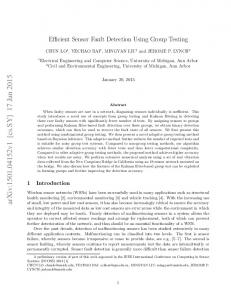
L Level Transducer Valve Flow Out
Flow In
Figure 1. Tank Example 3.1 System Dynamics This is a nonlinear system since the dynamics of the plant are dependent on the height of water level through the square root of the level. There also are some non-linearities due to the valve flow characteristics. This system can be modeled by F1 − F2 A where: L is the level of fluid in the tank F1 is the flow into the tank F2 is the flow out of the tank A is the area of the tank ∆L =
F2 = K ( t ) L
K ( t ) is the outlet flow resistance
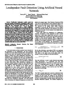
A change in level can be predicted if we measure both flows, but the actual level can only be predicted with the knowledge of both flows and the previous level. When a level sensor is drifting, this previous level is also in error so the drift cannot be detected. This is a case where although the correlation is extremely high, sensor drifts may not be detected. If the outlet flow resistance is a constant, the outlet flow is related to the square root of the level. In this case, the level can be predicted with the knowledge of the outlet flow rate through a non-linear correlation. A simulation of the case which has a random outlet flow resistance, is shown in Figure 2 and Figure 3 shows a simulation of case (2), which has a constant outlet flow resistance. These are designated as “fault free” and “noise free” data to both network architectures. Note that this simple example problem only has three sensors. The techniques described in this paper are usually applied to systems with 15-30 sensors. Therefore, the results may be sub-optimal when compared to larger systems.
3
Flow-In
1 0 .5 0
Flow-Out
0 .0 5
0 Level
40
0
1000
2000
3000
4000
0
1000
2000
3000
4000
0
1000
2000 T im e ( s e c )
3000
4000
20 0
Flow-In
Figure 2 System Dynamics with random outlet resistance
1 0 .5
Flow-Out
0 0 .0 6
0
1000
2000
3000
4000
0
1000
2000
3000
4000
0
1000
2000 T im e ( s e c )
3000
4000
0 .0 4 0 .0 2 Level
40 20 0
Figure 3 System Dynamics with constant outlet resistance The correlation coefficients, which indicate the linear relations among these parameters, are tabulated in Tables 1 and 2.
4
Parameter F1 F2 F1-F2 L0 L1 L0-L1
Table 1 Correlation Coefficients (CC) Matrix (random outlet resistance) F1 F2 F1-F2 L0 L1 L0-L1 1.0000 0.4918 0.9993 -0.3435 -0.3458 0.7389 0.4918 1.0000 0.4594 -0.0672 -0.0666 -0.1720 0.9993 0.4594 1.0000 -0.3475 -0.3499 0.7610 -0.3435 -0.0672 -0.3475 1.0000 1.0000 -0.1593 -0.3458 -0.0666 -0.3499 1.0000 1.0000 -0.1626 0.7389 -0.1720 0.7610 -0.1593 -0.1626 1.0000
Table 2 Correlation Coefficients (CC) Matrix (constant outlet resistance) Parameter F1 F2 F1-F2 L0 L1 L0-L1 1.0000 0.3885 0.9991 0.3975 0.3957 0.7845 F1 0.3885 1.0000 0.3483 0.9950 0.9949 -0.1878 F2 0.9991 0.3483 1.0000 0.3577 0.3558 0.8069 F1-F2 0.3975 0.9950 0.3577 1.0000 1.0000 -0.1956 L0 0.3957 0.9949 0.3558 1.0000 1.0000 -0.1976 L1 0.7845 -0.1878 0.8069 -0.1956 -0.1976 1.0000 L0-L1 Note: F1 is Inlet Flow, F2 is Outlet Flow; L0 is current level; L1 is 1 second delayed level In the case of randomly changing outlet flow resistance with time, there is a mostly random relationship between the water level L0 and the outlet flow F2 (CC=-0.0666). Furthermore, the water level is only partially correlated with the inlet flow F1 (CC=-0.3458). The same relationship exists for the delayed water level signal L1. This shows that there are no highly correlated relationships among the inlet flow, outlet flow, current water level, and delayed water level, except the current and delayed water level signals are highly correlated which is true in nature. The delayed signal provides no information on improving the correlation relationship. This shows that there is a lack of redundancy in such a system. However, in the case of time-invariant constant outlet flow resistance, there is a strong relationship between the outlet flow F2 and the water level L0 (CC=0.995). F2 can be predicted by knowing the value of L0 and vise versa. Also there is a relative high correlation between the change of level (L0-L1) and the inlet flow F1 (CC=0.7845), which means that the induced delayed level signal might help predicting the inlet flow. In such a case, the time delay neural network might have a better performance for predicting inlet flow F1. These expectations will be verified with the following experiment. 3.3 Network Architecture The basic feature of an AANN is that its output parameters are trained to equal to its input parameters, thus the number of input nodes equals the number of output nodes. The optional number of hidden layers and number of nodes is experimentally determined. The TDNN uses not only the current sensor measurement, but also the previous value as the inputs to the network. This gives the network temporal information. For this tank system, the MLP uses the current inlet flow, outlet flow and water level as network inputs, while the TDNN uses not only the above parameters, but also one or more previous values of the above parameters as network inputs. The internal network architecture of both networks has 1 hidden layer with 7 hidden nodes using logistic activation functions. The linear activation function is used in the output layer. The networks are trained with a Levenberg-Marquardt algorithm. Network performance was evaluated with a selected testing set
5
using normal data. The mean square error between the actual and network estimates is used for performance comparison. A robust training technique is used [Wrest et al, 1996]. 3.4 Network Training Algorithm A set of initial training data is used to start the training of the networks. After the training error goal has been reached, the network is tested with the test data. If the test set error goal has been reached, the network training process is done, otherwise, add the test data with the largest sum square error (SSE) into the training data set to form a new training data set, and the remaining test data set forms the new test data set. Repeat the above process until both the training and test error goals are met. In this research, the initial training data set was selected randomly. It is composed of 7% of the total data set, and the remaining 93% of total data is designated as the initial testing data. Figure 4 shows the hierarchy of the training paradigm. n e tw o r k I n itia liz e
T r a i n
n o
T r a i n i n g
tr a in in g
w e i g h ts
n e tw o r k
e r r o r
g o a l m e t?
y e s
T e s t n e tw o r k u s i n g t e s t d a t a
M
n e t w o r k
a x ( te s t d a ta
S S E )