Sensorless Battery Internal Temperature Estimation using a ... - arXiv

1

Sensorless Battery Internal Temperature Estimation using a Kalman Filter with Impedance Measurement

arXiv:1501.06160v1 [cs.SY] 25 Jan 2015

Robert R. Richardson and David A. Howey, Member, IEEE

Abstract—This study presents a method of estimating battery cell core and surface temperature using a thermal model coupled with electrical impedance measurement, rather than using direct surface temperature measurements. This is advantageous over previous methods of estimating temperature from impedance, which only estimate the average internal temperature. The performance of the method is demonstrated experimentally on a 2.3 Ah lithium-ion iron phosphate cell fitted with surface and core thermocouples for validation. An extended Kalman filter, consisting of a reduced order thermal model coupled with current, voltage and impedance measurements, is shown to accurately predict core and surface temperatures for a current excitation profile based on a vehicle drive cycle. A dual extended Kalman filter (DEKF) based on the same thermal model and impedance measurement input is capable of estimating the convection coefficient at the cell surface when the latter is unknown. The performance of the DEKF using impedance as the measurement input is comparable to an equivalent dual Kalman filter using a conventional surface temperature sensor as measurement input. Index Terms—Lithium-ion battery, impedance, temperature, thermal model, Kalman filter, state estimation.

I. I NTRODUCTION HE sustainable development of transportation relies on the widespread adoption of electric vehicle (EV) and hybrid electric vehicle (HEV) technology. Lithium-ion batteries are suitable for these applications due to their high specific energy and power density. However, their widespread deployment requires reliable on-board battery management systems to ensure safe and optimal performance. In particular, accurate on-board estimation of battery temperature is of critical importance. Under typical operating conditions, such as a standard vehicle drive cycle, cells may experience temperature differences between surface and core of 20 ◦ C or more [1]. High battery temperatures could trigger thermal runaway resulting in fires, venting and electrolyte leakage. While such incidents are rare [2], consequences include costly recalls and potential endangerment of human life. The conventional approach to temperature estimation is to use numerical electrical-thermal models [3], [4], [5], [6], [7]. Such models rely on knowledge of the cell thermal properties, heat generation rates and thermal boundary conditions. Models without online sensor feedback are unlikely to work in practice since their temperature predictions may drift from the true values due to small uncertainties in measurements and

T

The authors are with the Department of Engineering Science, University of Oxford, Oxford, UK, e-mail: {robert.richardson, david.howey} @eng.ox.ac.uk. c 2015 IEEE Copyright

parameters. However, using additional online measurements typically of the cell surface temperature and of the temperature of the cooling fluid - coupled with state estimation techniques such as Kalman filtering, the cell internal temperature may be estimated with high accuracy [4], [5], [6], [7]. However, large battery packs may contain several thousand cells [8], and so the requirement for surface temperature sensors on every cell represents substantial instrumentation cost. An alternative approach to temperature estimation uses electrochemical impedance spectroscopy (EIS) measurements at one or several frequencies to directly infer the internal cell temperature, without using a thermal model [9], [10], [11], [12], [13]. This exploits the fact that impedance is related to a type of volume averaged cell temperature, which we define later in this article. For brevity, we refer to the use of impedance to infer such a volume-averaged temperature as ‘Impedance-Temperature Detection’ (ITD). This has promise for practical application, since methods capable of measuring EIS spectra using existing power electronics in a vehicle or other application have been developed [14], [15], [16]. However, just like conventional surface temperature sensors, ITD alone does not provide a unique solution for the temperature distribution within the cell. Our previous work showed that by combining ITD with surface temperature measurements the internal temperature distribution could be estimated [17]. However, this approach still requires each cell to be fitted with a surface temperature sensor. Moreover, whilst the ITD technique was validated under constant coolant temperature conditions, the accuracy of the technique may be reduced if the temperature of the cooling medium is varied rapidly, as discussed in Section IV. Thus, if the cell electrical/thermal properties are known or can be identified, this information can be exploited to improve the estimate of the thermal state of the cell or reduce the number of sensors required. In this study we demonstrate that ITD can be used as the measurement input to a thermal model in order to estimate the cell temperature distribution. First, an extended Kalman filter (EKF) is used to estimate the cell temperature distribution when all the relevant thermal parameters, including the convection coefficient, are known. The thermal model consists of a polynomial approximation (PA) to the 1D cylindrical heat equation. The measurement input consists of the cell current and voltage, along with periodic measurements of the real part of the impedance at a single frequency. Second, a dual extended Kalman filter (DEKF) is used to identify the convection coefficient online when the latter is not known. The predicted core and surface temperatures in each case are validated against core and surface thermocouple measurements, with

2

agreement to within 0.47 ◦ C (2.4% of the core temperature increase). The performance of the combined thermal model plus ITD estimator is comparable to the performance of the same thermal model coupled with conventional surface temperature measurements. Table I shows the present study in the context of existing temperature estimation techniques, which highlights that this is the first study to use impedance as the measurement input to a thermal model. Study

Model

Forgez et al. [3] Lin et al. [5], [7] Kim et al. [6], [4] Srinivasan et al. [12], [9] Raijmakers et al. [11] Richardson et al. [17] Present study

X X X

X

Measurement Tsurf ITD X X X X X X X X

Table I C OMPARISON OF ONLINE TEMPERATURE ESTIMATION TECHNIQUES .

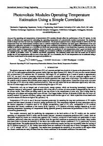
II. M EASUREMENT P RINCIPLE The electrochemical impedance, Z (ω) = Z 0 (ω)+jZ 00 (ω), of lithium ion cells is a function of temperature, state of charge (SOC) and state of health (SOH). Within an appropriate frequency range, however, the dependence on SOC and SOH is negligible and the impedance can thus be used to infer information about the cell temperature [12]. Previous ITD studies have used as a temperature-dependent parameter the real part of the impedance at a specific frequency [10], the phase shift at a specific frequency [12], [9], and the intercept frequency [11]. To demonstrate our technique we use the real part of the impedance at f = 215 Hz. Our previous work showed that the real part of the cell admittance (the inverse of the cell impedance) at 215 Hz can be related to the temperature distribution using a second order polynomial fit. For an annular cell with inner radius ri and outer radius ro the real part of the admittance is given by [17]: ˆ ro
2 Y0 = 2 r a1 + a2 T (r) + a3 T 2 (r) dr (1) ro ri where a1 , a2 and a3 are the 1st, 2nd and 3rd coefficients of the polynomial relating impedance to uniform cell temperature 2 (Y 0 = a1 + a2 Tunif orm + a3 Tunif orm ), provided that the admittivity varies in the radial direction only. This assumption is valid if the heat transfer from the top and bottom ends of the cell is negligible, which is approximately true for cylindrical cells connected in series with identical cells on either end [18], a configuration which may apply to the majority of cells in a large battery pack. However, the application of this approach to cooling configurations involving substantial end cooling would require a more involved expression for the admittance than eq. 1, as well as an appropriate modification to the 1D thermal model described in the following section. Moreover, although the method is applied to a cylindrical cell, the proposed approach could be applied to other geometries in a similar fashion. The polynomial fit (Fig. 1) was obtained

700 600

Data Fit: a1 T2 + a2 T + a3

Y’ / Ω−1

500 400 300 200 100 0

10

20 T (°C)

30

40

Figure 1. Polynomial fit to experimental data of admittance at f = 215 Hz vs. uniform cell temperature.

by offline impedance measurements on the cell at multiple uniform temperatures [17]. ITD can be viewed as identifying an EIS-based volume average temperature T EIS , which is defined as the uniform cell temperature that would give rise to the measured EIS1 . Thus the impedance input is similar to a conventional temperature measurement since it is a scalar function of the internal temperature distribution but does not uniquely identify the temperature distribution. Either measurement can therefore be used in conjunction with a thermal model, as shown in Fig. 2, to estimate core temperature.

a

b

Figure 2. Schematic of (a) the conventional approach to temperature estimation and (b) the proposed approach based on ITD.

III. T HERMAL -I MPEDANCE M ODEL A. Thermal Model The cell thermal model consists of the heat equation for 1D unsteady heat conduction in a cylinder, given by the following Boundary Value Problem (BVP) [2]: ρcp

∂ 2 T (r, t) kt ∂T (r, t) Q(t) ∂T (r, t) = kt + + ∂t ∂r2 r ∂r Vb

(2a)

where ρ, cp and kt are the density, specific heat capacity and thermal conductivity respectively, Vb is the cell volume, and Q is the heat generation rate. The boundary conditions are given 1 Note that, since the impedance temperature relationship is non-linear (as demonstrated in [19]), the EIS-based volume average temperature, T EIS , is not necessarily equal to the volume average temperature, T . Although, it should also be noted that the two are typically close in value, particularly if the temperature variation within the cell is small.

3

by: ∂T (r, t) ∂r

= − r=ro

∂T (r, t) ∂r

h (T (ro , t) − T∞ (t)) kt

(2b)

x˙ = Ax + Bu =

0

(2c)

∂UOCV (3) ∂T which is a simplified version of the expression first proposed by Bernardi et al [20]. The first term is the heat generation due to ohmic losses in the cell, charge transfer overpotential and mass transfer limitations. The current I and voltage V for this expression are measured online. The open circuit voltage UOCV is a function of SOC but is approximated here as a constant value measured at 50 % SOC, since the HEV drive cycles employed in this study operate the cell within a small range of SOC (47 − 63 %) and therefore OCV variation. If necessary, an estimator of UOCV could also be constructed (for example using a dynamic electrical model [21]), but for clarity and brevity we neglect this here. The second term, the entropic heat, is neglected in this study because (i) the term ∂Uavg /∂T is small (0 < ∂Uavg /∂T < 0.1 mVK-1 ) within the operated range of SOC [3], and (ii) the net reversible heat would be close to zero when the cell is operating in HEV mode. Q = I(V − UOCV ) + IT

B. Polynomial Approximation A polynomial approximation (PA) is used to approximate the solution of eq. 2a. The approximation was first introduced in [6] and is described in detail in that article, although the essential elements are repeated here for completeness. The model assumes a temperature distribution of the form  2  4 r r T (r, t) = a(t) + b(t) + d(t) (4) ro ro The two states of the model are the volume averaged temperature T and temperature gradient γ:  ˆ ro ˆ ro  2 2 ∂T T = 2 rT dr, γ= 2 r dr (5) ro 0 ro 0 ∂r The temperature distribution is expressed as a function of T , γ, and the cell surface temperature, Tsurf : 15ro − 3T − γ 8

T (r, t) = 4Tsurf    2 15ro r + −18Tsurf + 18T + γ 2 ro    4 45ro r + 15Tsurf − 15T − γ 8 ro

(6)

Using 2b, the surface temperature can be expressed as 24kt 15kt ro ro h T+ γ+ T∞ (7) 24kt + ro h 48kt + 2ro h 24kt + ro h

(8)

y = Cx + Du

r=0

where T∞ is the temperature of the heat transfer fluid, and h is the convection coefficient. A commonly employed expression for the heat source in a lithium ion battery is

Tsurf =

By obtaining the volume-average of eq. 2a and of its partial derivative with respect to r, a two-state thermal model consisting of two ODEs is obtained:

 T T T where x = T γ , u = [Q T∞ ] and y = [Tcore Tsurf ] are state, inputs and outputs respectively. The system matrices A, B, C, and D are defined as: " # −48αh −15αh ro (24kt +ro h) −320αh ro2 (24kt +ro h)

A= " B=

0 "

C= " D=

α kt Vb

24kt +ro h −120α(4kt +ro h) 2 ro (24kt +ro h)

48αh ro (24kt +ro h) 320αh ro2 (24kt +ro h)

#

120ro kt +15ro2 h 24kt −3ro h − 8(24k 24kt +ro h t +ro h) 24kt 15ro kt 24kt +ro h 48kt +2ro h # oh 0 24k4rt +r oh h 0 24krto+r oh

#

(9)

where α = kt /ρcp is the cell thermal diffusivity. C. Impedance Measurement Eq. 1 applies to an annulus with inner radius ri and outer radius ro . If the inner radius is sufficiently small, the cell may be treated as a solid cylinder, and eq. 1 becomes ˆ r0
2 r a1 + a2 T (r) + a3 T 2 (r) dr (10) Y0 = 2 ro 0 Substituting eq. 6 in eq. 10, the real admittance can be expressed as a function of of Tsurf , T , and γ 2

2 Y 0 = a1 + a2 T + 3a3 T + 2a3 Tsurf − 4a3 T Tsurf

+

15a3 ro2 γ 2 15a3 ro T γ 15a3 ro Tsurf γ (11) + − 32 8 8

Noting from eq. 7 that Tsurf is itself a function of T , γ and T∞ and the cell parameters, admittance is ultimately a function of T and γ, along with the known thermal parameters and environmental temperature. In other words, for known values of ro , kt , cp , ρ, and h, the impedance is a function of the cell state and T∞ , thus: Z 0 = f (T , γ, T∞ )

(12)

IV. F REQUENCY D OMAIN A NALYSIS In this section we analyze the error associated with the polynomial approximation, by comparing the frequency response of the PA model to the frequency response of a full analytical solution of eq. (2a). We also examine the approximation employed in [17], which used a combination of impedance and surface temperature measurements but no thermal model. To achieve a unique solution in that case, it was necessary to impose the assumption of a quadratic solution to the temperature distribution, and so we refer to this here as the ‘quadratic assumption’ (QA) solution.

4

As in [6], the frequency response function of the PA thermal system, H(s), is calculated by H(s) = D + C(sI − A)−1 B

(13)

where s = jω and I is the identity matrix. The frequency response of the analytical model is derived in [22], and that of the QA solution is derived in Appendix A.

Magnitude / dB

0 −30 −60 2

Error / dB

0

H11(s) = Tcore(s) / Q(s) Error / dB

Magnitude / dB

30

0

−2

10

0 −20 −40

−10 −15 H12 = Tcore(s) / T∞(s) 10 0 −10 −4 10 0

0

10

Magnitude / dB

Magnitude / dB

−2 −4 10 20

−5

−5

H22(s) = Tsurf(s) / T∞(s)

Error / dB

Error / dB

0.5

0 −0.5 −4 10

−2

10

Analytical Polynomial approx. Qaudratic assumption

−10

H21(s) = Tsurf(s) / Q(s) 0.5

−3

10

−2

0

10 10 Frequency (Hz)

0 −0.5 −4 10

−3

10 Frequency (Hz)

−2

10

Figure 3. Comparison of frequency responses of (i) analytical solution to the 1D cylindrical heat transfer problem, (ii) the polynomial approximation used in the current study and (iii) the quadratic assumption used in [17].

Fig. 3 shows the impact of changes in heat generation on Tcore and Tsurf (H11 and H21 respectively), and the impact of changes in cooling fluid temperature T∞ on Tcore and Tsurf (H12 and H22 respectively), for each model along with the error relative to the analytical solution. The results in these plots were obtained using the thermal parameters of the 26650 cell used in the present study (Table II). The response of H11 and H21 for both the PA and QA models are in good agreement with the analytical solution (note that the error in the response of H21 and H22 for the QA model is 0 since it takes the measured surface temperature as one of its inputs). However, the responses for both cases to changes in T∞ are less satisfactory. In particular, the response H12 for the QA model shows a rapid increase in error relative to the analytical solution at frequencies above ∼ 10−3 Hz. The PA performs well up to higher frequencies, although its error in H21 and H22 become unsatisfactory above ∼ 10−2 Hz. However, the frequency range at which the PA agrees with the analytical solution is broader than that of the QA model, and is considered satisfactory given the slow rate at which the cooling fluid temperature fluctuates in a typical battery thermal management system. V. E XPERIMENTAL Experiments were carried out with a 2.3 Ah cylindrical cell (A123 Model ANR26650 m1-A, length 65 mm, diameter 26

mm) with LiFePO4 positive electrode and graphite negative electrode. The cell was fitted with two thermocouples, one on the surface and another inserted into the core via a hole which was drilled in the positive electrode end (Fig. 4). Cell cycling and impedance measurements were carried out using a Biologic HCP-1005 potentiostat/booster. The impedance was measured using Galvanostatic Impedance Spectroscopy with a 200 mA peak-to-peak perturbation current. The environmental temperature was controlled with a Votsch VT4002 thermal chamber. The chamber includes a fan which operates continuously at a fixed speed during operation. In order to calibrate the impedance against temperature, EIS measurements were first conducted on the cell in thermal equilibrium at a range of temperatures. These experiments and the subsequent identification of the polynomial coefficients a1 , a2 , and a3 are described in [17]. Dynamic experiments were then conducted using two 3500 s current excitation profiles - the first to parameterise the thermal model, and the second to validate the identified parameters and to demonstrate the temperature estimation technique. The profiles were generated by looping over different portions of an Artemis HEV drive cycle. The applied currents were in the range −23 A to +30 A. For the duration of the experiments, single frequency (215 Hz) impedance measurements were carried out every 24 s and the surface and internal temperatures were also monitored. In order to minimise heat loss through the cell ends, these were insulated using Styrofoam (Fig. 4). Before each experiment, the SOC was adjusted to 50% by drawing a 0.9 C current. The temperature of the thermal chamber was set to 8 ◦ C and the cell was allowed to rest until its temperature equilibrated before experiments began. Besides being a function of temperature and SOC, the impedance is also a function of DC current, mainly due to the charge transfer polarization decreasing with increasing current [23]. Previous results confirmed that when the EIS perturbation current is superposed over an applied DC current, the impedance measurement is altered [17]. To overcome this, the cell was allowed to rest briefly for 4 s before each EIS measurement was taken, i.e. 20 s periods of the excitation current followed by 4 s rests. The duration of this rest period was kept as short as possible to ensure that the thermal response of the cell to the applied cycle was not significantly altered, and it was found that the core cell temperature dropped by at most 0.25◦ C during these rest periods. The issue of impedance measurement under DC current warrants further investigation. VI. M ODEL PARAMETERISATION & VALIDATION Parameterisation is performed to estimate the values of kt , cp , and h. The density ρ was identified in advance by measuring the cell mass and dividing by its volume. The values from the first excitation profile (comprising cell current, voltage plus surface, core and chamber temperatures) were used for the estimation. The parameterisation was carried out offline using fminsearch in Matlab to minimise the magnitude of the Euclidean distance between the measured and estimated core and surface

5

a

Temperaturedsensors (fordvalidation): Tcore , Tsurf

all of these studies), heat generation in the contact resistances between the cell and connecting wires and/or measurement uncertainty in the temperature. The convection coefficient is within the range expected of forced convection air cooling [24].

Thermaldchamber

Parameter

Units

Reference

Initial

Identified

ρ

kg m-3

-

2107

cp

J kg-1 K-1

1050

1171.6

kt

W m-1 K-1

0.55

0.404

h

W m-2

2047-2118 [4], [25], [26] 1004.9-1109.2 [3], [7], [4] 0.488-0.690 [22], [25], [4] -

20

39.3

40 20 0 -20 -40

20 10

0

500

1000

1500

2000

0

td(s)

Powerdsupplydvdimpedance

b

Table II C OMPARISON OF REFERENCE & ESTIMATED PARAMETERS

30 T

Id(A)

e-

500

1000 td(s)

1500

2000

Datadacquisitiondmodule

c

The measured core and surface temperatures (subscript ‘exp’) and the corresponding model predictions (subscript ‘m’) for the parameterised model are shown in Fig. 5. The root-mean-square errors (RMSE) in the surface and core temperatures are 0.19 ◦ C and 0.18 ◦ C respectively. 30

T / °C

25 20 15 10

Tcore,exp

Tcore,m

Tsurf,exp

Tsurf,m

5 0

d

500

1000

1500 2000 time / s

2500

3000

3500

Figure 5. Model parameterisation: Comparison between measured and predicted core and surface temperatures in the parameterised model.

The model with identified parameters was validated against the second current excitation profile (Fig. 6). The RMSEs in the core and surface temperatures were 0.21 ◦ C and 0.16 ◦ C respectively in this case. These errors are only marginally greater than those in the parameterisation test, indicating that the estimation is satisfactory. 30

T / °C

25

Figure 4. Experimental setup for parameter identification and validation. (a) schematic diagram with cutaway view showing cell core and jelly roll, (b) cell drilling procedure, (c) prepared cell inside thermal chamber, (d) power supply & thermal chamber.

temperatures, as in [4]. Table II compares the identified parameters with the initial guesses and parameters for the same cell from the literature. The estimated parameters are close to those reported in the literature. The deviations may be attributed to manufacturing variability, error in the heat generation calculation (due to the omission of entropic heating in

20 15

Tcore,exp

Tcore,m

10

Tsurf,exp

Tsurf,m

5 0

500

1000

1500 2000 time / s

2500

3000

3500

Figure 6. Model validation. Comparison between measured and predicted core and surface temperatures in the parameterised model applied to the second current excitation profile.

VII. S TATE E STIMATION Kim et al. [6] showed that the effect of changes to the value of h on the predicted surface and core temperatures is greater

6

than the effect of changes to the other thermal parameters. Moreover, h depends strongly on the thermal management system settings and its calculation often relies on empirical correlations between coolant flow rates and heat transfer. Thus, there is a need to identify the convection coefficient online during operation. This section outlines the use of a dual extended Kalman filter (DEKF) [27] for estimating the core and surface temperatures and the convection coefficient. The DEKF reduces to an EKF if the convection coefficient is assumed known and provided to the model in advance. We firstly modify eq. 9 by rewriting it as a discrete time model, setting the impedance as the model output, and explicitly including the dependency on the parameter, hk : ¯ k )xk + B(h ¯ k )uk + vk xk+1 = A(h yk = f (xk , hk ) + nk

(14) (15)

hk+1 = hk + ek

(16)

where yk = Z 0 and f (xk , hk ) is the non-linear function relating the state vector to the measurement (i.e. eq. 12), and vk , nk and ek are the noise inputs of the covariance matrices Rv , Rn and Re . The states, inputs and measured T  T outputs are thus x = T γ , u = [Q T∞ ] and y = Z 0 . Note that, although the impedance is now the model output, the core and surface temperatures are also computed from the identified states and parameter at each time step using eq. 8, ¯ and for validation against the thermocouple measurements. A ¯ B are system matrices in the discrete-time domain, given by ¯ = e(A∆t) , B ¯ = A−1 (A ¯ − I)B A

(17)

where ∆t is the sampling time of 1 s. The update processes are then given as follows. The time update processes for the parameter filter are: ˆ− = h ˆ k−1 h k (Pkh )−

=

h Pk−1

+R

e

k−1

k−1

(29)

where Hkh is the Jacobian matrix of partial derivatives of f with respect to h: ∂f (xk , hk ) h (30) Hk = ∂hk ˆ− hk =hk

The above algorithm can be simplified to a standard EKF by omitting the parameter update processes (eqs. 16, 18-19 and 27-30) and assuming the convection coefficient is fixed. In the following section we investigate the performance of both the baseline EKF and the full DEKF algorithm. VIII. R ESULTS We first investigate the performance of an EKF estimator whereby the convection coefficient is provided and assumed fixed. We then compare the performance of the DEKF algorithm with that of the baseline EKF when an incorrect initial estimate of the convection coefficient is provided. Lastly, we compare the performance of the DEKF with that of a dual Kalman filter (DKF) based on the same thermal model but with Tsurf as the measurement input rather than Z 0 .

The initial state estimate provided to the battery is x ˆ0 = [25 0], i.e. the battery has a uniform temperature distribution at 25 ◦ C. The true initial battery state is a uniform temperature distribution at 8 ◦ C. The covariance matrices are calculated as Rn = σn2 and Rv = βv2 diag(2, 2). The first tuning parameter is chosen as σn = 1 × 10−4 Ω, which is a rough estimate of the standard deviation of the impedance measurement. The second tuning parameter was chosen as βv = 0.1, by trial and error. Fig. 7 shows that, using the EKF, the core and surface temperatures quickly converge to the correct values and are accurately estimated throughout the entire excitation profile. The RMSEs of core and surface temperature are 1.35 ◦ C and 1.34 ◦ C respectively. In contrast, the RMSEs for the open loop model (subscript ‘m’) with no measurement feedback are 6.66 ◦ C and 4.42 ◦ C respectively. It should be noted that since the uncertainty of the impedance measurement typically increases as impedance decreases, the temperature estimates could be more uncertain at higher temperatures. Hence, the implementation of this technique could be more challenging at higher ambient temperature conditions than those studied here. It should be noted that we also achieved similar performance using a simpler EKF based on Z 0 with the assumption that

(20) (21)

h=hk

Since the relationship between impedance and the cell state is non-linear, the measurement model must be linearised about the predicted observation at each measurement. The measurement update equations for the state filter are:
−1 x Kxk = (Pxk )− (Hxk )T Hxk (Pxk )− (Hk )T + Rn (23)   x ˆ− ˆk = x ˆ− x x− (24) k + Kk zk − f (ˆ k , hk ) Pxk = (I − Kxk Hxk )(Pxk )−

Pkh = (I − Kkh Hkh )(Pkh )−

A. Convection Coefficient Known

where x ˆ− ˆk are the a priori and a posteriori estimates k and x of the state, and (Pxk )− and Pxk−1 are the corresponding error ¯ k−1 and B ¯ k−1 are calculated by: covariances. The matrices A ¯ k−1 = A(h) ¯ ¯ k−1 = B(h) ¯ ˆ− , B ˆ− A (22) h=hk

The measurement update processes for the parameter filter are:
−1 Kkh = (Pkh )− (Hkh )T Hkh (Pkh )− (Hkh )T + Rn (27)   ˆk = h ˆ − + K h zk − f (ˆ ˆ −) h xk , h (28) k k k

(19)

ˆ k are the a priori and a posteriori estimates of where and h h are the corresponding the parameter h, and (Pkh )− and Pk−1 error covariances. The time update processes for the state filter are:

k

xk =ˆ xk

(18)

ˆ− h k

¯ ¯ k−1 uk−1 ˆ− ˆ k−1 + B x k = Ak−1 x x − x T ¯ ¯ (P ) = Ak−1 P A + Rv

where Kxk is the Kalman gain for the state, and Hxk is the Jacobian matrix of partial derivatives of f with respect to x: ∂f (xk , hk ) x (26) Hk = ∂xk −

(25)

7

45

27

17 40

25

15

35

error / °C

16

(Tcore,EKF − Tcore,exp)

(Tcore,DEKF − Tcore,exp)

2 0

30

T / °C

4

0

25

500

1000

1500

2000

2500

3000

3500

45 20

40

15

5

0

500

Tcore,exp

TTcore,m core,m

Tcore,EKF

Tsurf,exp

TTsurf,m surf,m

Tsurf,EKF

1000

1500

2000

2500

3000

20

16

30

3500

T / °C

10

22

18

35

25 20

Time / s 15

Figure 7.

Temperature results for EKF using

Z0

10

as measurement input

5

Tcore,EKF

Tcore,DEKF

T

Tsurf,EKF

Tsurf,DEKF

surf,exp

0

500

1000

1500

2000

2500

3000

3500

100 h / Wm−2k−1

the impedance is related directly to T rather than to T EIS . However, this assumption may lead to unsatisfactory results for cells with a larger radius or when larger temperature gradients exist within the cell. Moreover, since this approach assumes that the impedance is a function of the state only (and not the parameter h), it is not suitable for the application of the DEKF discussed in the following section.

Tcore,exp

80 htrue

60

hEKF

hDEKF

40 20

0

500

1000

1500

2000

2500

3000

3500

t/s

Figure 8.

Temperature results for DEKF using Z 0 as measurement input

B. Convection Coefficient Unknown Next we investigate the performance of the DEKF. The same incorrect initial state estimate is provided to the battery, x ˆ0 = [25 0]. Moreover, an incorrect initial estimate for the ˆ 0 = 2 × htrue . This convection coefficient is provided, h value of h is also provided to the EKF. The error covariance matrix for the parameter estimator is Re = βe2 where the tuning parameter is chosen as βe = 2.5. Fig. 8 compares the results of both of these cases against the thermocouple measurements. The EKF is shown to overestimate the core temperature and underestimate the surface temperature for the duration of the experiments. This is expected, since the impedance measurement ensures the accuracy of the volume averaged cell temperature but the model assumes that the convection coefficient is higher than in reality, and therefore the temperature difference across the cell is overestimated. In contrast, the DEKF corrects the convection coefficient, and thus improves the accuracy of the subsequent temperature predictions. This is evident from the errors in the core temperature estimate (top plot of Fig. 8), which initially are similar in both cases but drop to much smaller values for the DEKF once the correct convection coefficient is identified. The RMSEs of core and surface temperature in each case are shown in Table III, along with the values for the time period, 1200 < t < 3500 s (i.e. after the convection coefficient value has converged). Finally, we investigate the case where Tsurf is used as the measurement (y = Tsurf ) to the estimator rather than Z 0 . This results in a linear KF and DKF exactly equivalent to that studied in [4]. The tuning parameters for the covariance matrices are also chosen to be the same as those employed in [4]. The same initial state and parameter estimates are provided as for the DEKF. Fig. 9 shows that the standard

EKF in this case overpredicts the core temperature by a greater margin than the EKF based on Z 0 , although the surface temperature estimate is much more accurate. This is because the surface thermocouple ensures an accurate surface temperature estimate and to reconcile this with the overestimated convection coefficient, the core temperature estimate is forced to be much greater. The DKF correctly identifies the correct convection coefficient, in the same way as the DEKF. Since the thermocouple measurement exhibits less noise than the impedance measurement, the model converges to the correct estimate for h more quickly than in the DEFK case, as shown by the RMSE values in Table III. Method EKF + Z 0 KF + Tsurf DEKF + Z 0 DKF + Tsurf

0 < t < 3500 s Tcore Tsurf 2.04 2.06 2.49 1.44 1.43 1.24 0.36 0.33

1200 < t < 3500 s Tcore Tsurf 1.79 1.98 2.90 1.58 0.47 0.42 0.16 0.14

Table III C OMPARISON OF RMSE S FOR CORE AND SURFACE TEMPERATURES (◦ C) WITH UNKNOWN CONVECTION COEFFICIENT.

In conclusion, the temperature and convection coefficient estimators using Z 0 as measurement input are capable of accurately estimating the core and surface temperatures and the convection coefficient. The performance is comparable to that of an estimator using the same thermal model coupled with surface temperature measurements. Moreover, the performance of the present method is superior to that of previous methods based on impedance measurements alone, which only provide an estimate of the average internal temperature of the cell.

8

°

error / C

ACKNOWLEDGEMENTS 8 6 4 2 0 −2 0

(Tcore,EKF − Tcore,exp)

500

1000

1500

(Tcore,DEKF − Tcore,exp)

2000

2500

3000

3500

45 40

18

22

16

20

35 T / °C

30 25

A PPENDIX

20

A. Frequency Domain Analysis of Quadratic Assumption

15 10 5 0 h / Wm−2k−1

This work was funded by a NUI Travelling Scholarship, a UK EPSRC Doctoral Training Award and the Foley-Bejar scholarship from Balliol College, University of Oxford. This publication also benefited from equipment funded by the John Fell Oxford University Press (OUP) Research Fund. Finally, the authors would like to thank Peter Ireland and Adrien Bizeray for valuable comments, and Robin Vincent for the facilities to prepare the instrumented battery.

Tcore,exp

T

T

T

Tsurf,EKF

Tsurf,DEKF

500

1000

core,DEKF

core,EKF

surf,exp

1500

2000

2500

3000

3500

100 80 htrue

60

hEKF

hDEKF

40 20 0

500

1000

1500

2000

2500

3000

3500

t/s

Figure 9.

DKF using Tsurf as measurement input.

IX. C ONCLUSIONS Impedance temperature detection enables both core and surface temperature estimation without using temperature sensors. In this study, the use of ITD as measurement input to a cell thermal model is demonstrated for the first time. Previously, we estimated cell temperature distribution by combining ITD with a surface temperature measurement and imposing a quadratic assumption on the radial temperature profile. Frequency domain analysis shows that the QA solution may be inaccurate if the temperature of the cooling fluid has fluctuations on the order of 10−3 Hz or higher. The PA thermal model used in the present study is robust to higher frequency fluctuations (∼ 10−2 Hz). An EKF using a parameterised PA thermal model with ITD measurement input is shown to accurately predict core and surface temperatures for a current excitation profile based on an Artemis HEV drive cycle. A DEKF based on the same thermal model and measurement input is capable of accurately identifying the convection coefficient when the latter is not provided to the model in advance. The performance of the DEKF using impedance as measurement input is comparable to an equivalent DKF estimator using surface temperature as measurement input, although the latter is slightly superior due to the higher accuracy of the thermocouple. Future work will investigate the application of ITD to multiple cells in a battery pack, as well as investigating methods of combining impedance with conventional sensors to enable more robust temperature monitoring and fault detection, and self-calibration.

The analysis leading to the frequency response plots of the QA model in Fig. 3 is outlined in this section. The QA model was used in [17] to obtain a unique solution for the temperature distribution when the impedance and surface temperature were measured but the cell thermal properties and heat generation rates were assumed unknown. To achieve a unique solution in that case, it was necessary to impose the assumption of a quadratic temperature distribution based on the solution of the 1D heat equation at steady state. Muratori et al. [22] showed that the time domain PDE of eq. 2a, can be transformed into an equivalent ODE problem in the frequency domain which can be solved analytically. Using this approach the solution for the temperatures at the core and surface of the cell are shown to be: Tcore (s) =

1 Q(s) + kt a 2

Tsurf (s) =

1 Q(s) + kt a 2

1 h kt (T∞ (s) − ka2 Q(s)) h kt J0 (aro ) − aJ1 (aro ) h 1 kt (T∞ (s) − kt a2 Q(s)) h kt J0 (aro )

− aJ1 (aro )

(31) J0 (aro ) (32)

2

−1

where a = sα , Q(s) is the transform of Q(t), and Ji is the ith -order Bessel function of the first kind [28]. Eqs. 31 and 32 can be interpreted as the outputs of a continuous time dynamic system [22], where u(t) = [Q(t), T∞ (t)]T and y(t) = [Tcore (t), Tsurf (t)]T , such that the solution of the BVP is equivalent to the impulse response of the system:      Tcore (s) H11 (s) H12 (s) Q(s) = (33) Tsurf (s) H21 (s) H22 (s) T∞ (s) where the H matrix is formed by the transfer functions: H11 (s) = H12 (s) =

1 kt a2

h h kt J0 (aro ) − aJ1 (aro ) − kt h kt J0 (aro ) − aJ1 (aro ) h kt

h kt J0 (aro )

− aJ1 (aro ) 1 −aJ1 (aro ) H21 (s) = kt a2 kh J0 (aro ) − aJ1 (aro ) t H22 (s) =

h kt J0 (aro ) h kt J0 (aro )

− aJ1 (aro )

(34) (35) (36) (37)

This system of transfer functions gives frequency responses for the analytical solution results plotted in Fig. 3. Using a similar approach, we can develop an analytical solution to the

9

QA model used in [17], where we denote the new transfer function HQA (s). In this case, both the volume-averaged cell temperature (identified via the impedance2 ) and the surface temperature were measured directly, and it is assumed that no other information was available. Since these two inputs alone are not sufficient to achieve a unique solution for the temperature distribution, it was also necessary to impose the following constraint on the temperature profile:   r2 TQA (r) = Tsurf + (Tcore, QA − Tsurf ) 1 − 2 ro

T QA

ˆ

ro

rTQA (r)dr = T

(39)

0

Substituting eq. 38 in eq. 39 and integrating, the QA core temperature becomes Tcore, QA = 2T − Tsurf

(40)

Thus, an estimate for the core temperature is obtained directly from the surface and volume averaged temperature measurements. Since the surface temperature is measured, the values of HQA, 21 (s) and HQA, 22 (s) are identical to the corresponding values of the unsteady thermal model. The values of HQA, 11 (s) and HQA, 12 (s) can be obtained as follows: Substituting T from eq. 5 into eq. 40, the QA approximation of the core temperature can be expressed as a function of the temperature distribution: Tcore,QA

4 = 2 ro

ˆ

ro

(rT (r)dr − Tsurf ) dr

(41)

0

Substituting eqs. 31 and 32, for ´ r T (r) and Tsurf , respectively, and integrating (noting that 0 o rJ0 (ar)dr = ro J1 (aro )/a), we obtain: Q(s) + kt a2  1 h kt (T∞ (s) − kt a2 Q(s)) 4J1 (aro )

Tcore, QA =

h kt J0 (aro )

− aJ1 (aro )

aro

 − J0 (aro )

kt a2 ro J1 (aro ) − 2hro aJ0 (aro ) + 4hJ1 (aro ) kt ro a3 (hJ0 (aro ) − kt aJ1 (aro )) (44) 3 2 −hkt a J0 aro + 4hkt a J1 aro HQA, 21 (s) = (45) kt ro a3 (hJ0 aro − kt aJ1 (aro )) HQA, 12 (s) = H21 (s) (46)

HQA, 11 (s) = −

HQA, 22 (s) = H22 (s) (38)

This is the 1D steady-state solution of the heat equation for a cylinder with uniform heat generation [24], with T (r) and Tcore replaced by TQA (r) and Tcore, QA . The volume average of the QA temperature distribution is set equal to the true volume average temperature, giving: 2 = 2 ro

where the H matrix is formed by the functions:

(42)

Thus, the QA system model is given by:      Tcore, QA (s) HQA, 11 (s) HQA, 12 (s) Q(s) = Tsurf, QA (s) HQA, 21 (s) HQA, 22 (s) T∞ (s) (43) 2 As discussed in Section I, the impedance actually identifies T EIS , which is not necessarily equal to T . However, the assumption that T EIS = T is satisfactory for the purpose of identifying the frequencies at which errors relative to the analytical solution become significant, and is only used for this purpose in this article.

(47) R EFERENCES

[1] U. S. Kim, C. B. Shin, and C.-S. Kim, “Modeling for the scale-up of a lithium-ion polymer battery,” J. Power Sources, vol. 189, no. 1, pp. 841–846, Apr. 2009. [2] Q. Wang, P. Ping, X. Zhao, G. Chu, J. Sun, and C. Chen, “Thermal runaway caused fire and explosion of lithium ion battery,” J. Power Sources, vol. 208, pp. 210–224, Jun. 2012. [3] C. Forgez, D. Vinh Do, G. Friedrich, M. Morcrette, and C. Delacourt, “Thermal modeling of a cylindrical LiFePO4/graphite lithium-ion battery,” J. Power Sources, vol. 195, no. 9, pp. 2961–2968, May 2010. [4] Y. Kim, S. Mohan, S. Member, J. B. Siegel, A. G. Stefanopoulou, and Y. Ding, “The Estimation of Temperature Distribution in Cylindrical Battery Cells Under Unknown Cooling Conditions,” IEEE Trans. Control Syst. Technol., pp. 1–10, 2014. [5] X. Lin, H. E. Perez, J. B. Siegel, A. G. Stefanopoulou, R. D. Anderson, and M. P. Castanier, “Online Parameterization of Lumped Thermal Dynamics in Cylindrical Lithium Ion Batteries for Core Temperature Estimation and Health Monitoring,” IEEE Trans. Control Syst. Technol., vol. 21, no. 5, pp. 1745–1755, Sep. 2013. [6] Y. Kim, J. B. Siegel, and A. G. Stefanopoulou, “A computationally efficient thermal model of cylindrical battery cells for the estimation of radially distributed temperatures,” in American Control Conference (ACC), Washington, DC, 2013, pp. 698–703. [7] X. Lin, H. E. Perez, S. Mohan, J. B. Siegel, A. G. Stefanopoulou, Y. Ding, and M. P. Castanier, “A lumped-parameter electro-thermal model for cylindrical batteries,” J. Power Sources, vol. 257, pp. 1–11, Jul. 2014. [8] A. Pesaran, G. H. Kim, and M. Keyser, “Integration Issues of Cells into Battery Packs for Plug-In and Hybrid Electric Vehicles,” in EVS-Â24 International Battery, Hybrid and Fuel Cell Electric Vehicle Symposium, no. May, Stavanger, Norway, 2009. [9] R. Srinivasan, “Monitoring dynamic thermal behavior of the carbon anode in a lithium-ion cell using a four-probe technique,” J. Power Sources, vol. 198, pp. 351–358, Jan. 2012. [10] J. P. Schmidt, S. Arnold, A. Loges, D. Werner, T. Wetzel, and E. IversTiffée, “Measurement of the internal cell temperature via impedance: evaluation and application of a new method,” J. Power Sources, vol. 243, pp. 110–117, Jun. 2013. [11] L. Raijmakers, D. Danilov, J. van Lammeren, M. Lammers, and P. Notten, “Sensorless battery temperature measurements based on electrochemical impedance spectroscopy,” J. Power Sources, vol. 247, pp. 539–544, Feb. 2014. [12] R. Srinivasan, B. G. Carkhuff, M. H. Butler, and A. C. Baisden, “Instantaneous measurement of the internal temperature in lithium-ion rechargeable cells,” Electrochimica Acta, vol. 56, no. 17, pp. 6198–6204, Jul. 2011. [13] J. Zhu, Z. Sun, X. Wei, and H. Dai, “A new lithium-ion battery internal temperature on-line estimate method based on electrochemical impedance spectroscopy measurement,” Journal of Power Sources, vol. 274, pp. 990–1004, Jan. 2015. [14] D. A. Howey, P. D. Mitcheson, S. Member, V. Yufit, G. J. Offer, and N. P. Brandon, “On-line measurement of battery impedance using motor controller excitation,” IEEE Trans. Veh. Technol., vol. 63, no. 6, pp. 2557–2566, 2014. [15] N. Brandon, P. Mitcheson, D. A. Howey, V. Yufit, and G. J. Offer, “Battery Monitoring in Electric Vehicles, Hybrid Vehicles and other Applications,” 2012. [16] W. Huang and J. Abu Qahouq, “An Online Battery Impedance Measurement Method Using DC-DC Power Converter Control,” IEEE Trans. Ind. Electron., vol. 0046, no. c, pp. 1–1, 2014. [17] R. R. Richardson, P. T. Ireland, and D. a. Howey, “Battery internal temperature estimation by combined impedance and surface temperature measurement,” J. Power Sources, vol. 265, pp. 254–261, May 2014.

10

[18] M. Fleckenstein, O. Bohlen, M. a. Roscher, and B. Bäker, “Current density and state of charge inhomogeneities in Li-Ion battery cells with LiFePO4 as cathode material due to temperature gradients,” J. Power Sources, vol. 196, no. 10, pp. 4769–4778, Jan. 2011. [19] Y. Troxler, B. Wu, M. Marinescu, V. Yufit, Y. Patel, A. J. Marquis, N. P. Brandon, and G. J. Offer, “The effect of thermal gradients on the performance of lithium-ion batteries,” Journal of Power Sources, no. 247, pp. 1018–1025, Jun. 2013. [20] D. Bernardi, E. Pawlikowski, and J. Newman, “A General Energy Balance for Battery Systems,” J. Electrochem. Soc., vol. 132, no. 1, pp. 5–12, 1985. [21] C. R. Birkl and D. A. Howey, “Model identification and parameter estimation for LiFePO 4,” in IET Hybrid and Electric Vehicles Conference 2013 (HEVC 2013), 2013, pp. 1–6. [22] M. Muratori, N. Ma, M. Canova, and Y. Guezennec, “A Model Order Reduction Method for the Temperature Estimation in a Cylindrical Li-Ion Battery Cell,” ASME 2010 Dynamic Systems and Control Conference, Volume 1, no. 7, pp. 633–640, 2010. [23] B. Ratnakumar, M. Smart, L. Whitcanack, and R. Ewell, “The impedance characteristics of Mars Exploration Rover Li-ion batteries,” J. Power Sources, vol. 159, no. 2, pp. 1428–1439, Sep. 2006. [24] F. P. Incropera and D. P. De Witt, Fundamentals of Heat and Mass Transfer, 6th ed. Wiley, 2007. [25] H. Khasawneh, J. Neal, M. Canova, and Y. Guezennec, “Analysis of heat-spreading thermal management solutions for lithium-ion batteries,” in ASME 2011 International Mechanical Engineering Congress and Exposition, 2011, pp. 421–428. [26] X. Li, F. He, and L. Ma, “Thermal management of cylindrical batteries investigated using wind tunnel testing and computational fluid dynamics simulation,” J. Power Sources, vol. 238, pp. 395–402, Sep. 2013. [27] E. A. Wan and A. T. Nelson, “Dual extended Kalman filter methods.” in Kalman filtering and neural networks. New York, NY: Wiley, 2001, pp. 123–173. [28] E. Kreyszig, Advanced engineering mathematics. John Wiley & Sons, 2010.

Robert R. Richardson received the B.Eng. degree in mechanical engineering from the National University of Ireland, Galway, in 2012. He is currently working toward the D.Phil (PhD) degree in the Energy and Power Group, Department of Engineering Science, University of Oxford, Oxford, U.K, where his research is focused on impedance based battery thermal management.

David A. Howey (M’10) received the B.A. and M.Eng. degrees from Cambridge University, Cambridge, U.K., in 2002 and the Ph.D. degree from Imperial College London, London, U.K., in 2010. He is currently a Lecturer with the Energy and Power Group, Department of Engineering Science, University of Oxford, Oxford, U.K. He leads projects on fast electrochemical modeling, model-based battery management systems, battery thermal management, and motor degradation. His research interests include condition monitoring and management of electricvehicle electric-vehicle components.