A comparison of sensorless speed estimation methods for induction ...

Proceedings of the American Control Conference Anchorage, AK May 8-10, 2002

1

A Comparison of Sensorless Speed Estimation Methods for Induction Motor Control Marc Bodson and John Chiasson Abstract – Many different techniques have been proposed to estimate the speed of an induction motor without a shaft sensor. Three representative approaches are considered in the paper. The methods are compared in terms of their sensitivity to parameter variations, their ability to handle loads on the motor, and their speed tracking capability.

The usual implementation of field-oriented control assumes that the stator currents are measured, that a shaft sensor is used to obtain ω, and that the fluxes are estimated through integration of ˆ /dt = −ηψ ˆ − np ω ψ ˆ + ηM iSa dψ Ra Ra Rb ˆ /dt = −ηψ + np ω ψ ˆ + ηM iSb dψ Rb Rb Ra

Keywords – Sensorless Control, Induction Motor

I. Sensorless Control Methods A. Mathematical Model For reference, we begin with the mathematical model of the induction motor in terms of the variables θ, ω, ψ Ra , ψ Rb , iSa and iSb , as given by [17] dω/dt dψ Ra /dt dψ Rb /dt uSa uSb

= = = = =

np (M/JLR ) (iSb ψ Ra − iSa ψ Rb ) − τ L /J −(RR /LR )ψ Ra − np ωψ Rb + M (RR /LR )iSa −(RR /LR )ψ Rb + np ωψ Ra + M (RR /LR )iSb RS iSa + σLS diSa /dt + (M/LR )dψ Ra /dt RS iSb + σLS diSb /dt + (M/LR )dψ Rb /dt (1)

where σ , 1−M 2 /LR LS is the so-called leakage parameter. The system (1) can also be written in explicit state-space form as dω/dt dψ Ra /dt dψ Rb /dt diSa /dt diSb /dt

= = = = =

µ (iSb ψ Ra − iSa ψ Rb ) − τ L /J −ηψ Ra − np ωψ Rb + ηM iSa −ηψ Rb + np ωψ Ra + ηM iSb ηβψ Ra + βnp ωψ Rb − γiSa + uSa /σLS ηβψ Rb − βnp ωψ Ra − γiSb + uSb /σLS (2)

with η , RR /LR = 1/TR , β , M/σLR LS , µ , 2np M/nph JLR , γ , M 2 RR /σL2R LS + RS /σLS . In industrial settings where high-performance variable speed control is desired, field-oriented control (or one of its variants) is the algorithm of choice [17]. Field-oriented control is based on a coordinate system that rotates with the angle ρ q = tan−1 (ψ Rb /ψ Ra ). One lets ρ = tan−1 (ψ Rb /ψ Ra ),

ψ d = ψ 2Ra + ψ 2Rb and the currents and voltages are then transformed into the new coordinate system as ¸ · ¸ · ¸· cos(ρ) sin(ρ) id iSa , iq iSb − sin(ρ) cos(ρ) · ¸ · ¸ ¸· ud cos(ρ) sin(ρ) uSa , uq uSb − sin(ρ) cos(ρ) M. Bodson is with the ECE Department, University of Utah, Salt Lake City, UT 84112, [email protected]. J. Chiasson is with the ECE Department, University of Tennessee, Knoxville, TN 37996, [email protected]

0-7803-7298-0/02/$17.00 © 2002 AACC

(3)

ˆ )2 + A straightforward calculation shows that (ψ Ra − ψ Ra 2 ˆ (ψ Rb − ψ Rb ) → 0, so that (3) provides a stable estimate of the fluxes. The flux estimate is crucial to this approach even if only torque (as opposed to speed) control is required. This estimator depends on knowing the parameter η , RR /LR = 1/TR , that is, the reciprocal of the rotor time constant. Due to ohmic heating, this parameter varies, throwing off the flux estimate and consequently the determination of the angle ρ = tan−1 (ψ Rb /ψ Ra ). Quite a bit of research has been devoted to making field-oriented control adaptive to the rotor time constant, assuming that a shaft sensor is available, as given in the work [18] [20] and the references therein. In contrast, the (ultimate) objective of sensorless control is to achieve adaptation to unknown speed as well as to motor parameters. B. Method 1: Adaptive Method One approach to the sensorless control problem is to consider the speed as an unknown “constant” parameter and to use the techniques of adaptive control to estimate this parameter [22] [23] [25]. The idea is that the speed changes slowly compared to the electrical variables. This approach was first formulated by Shauder [25], with important modifications proposed by Peng and Fukao [22]. Specifically, using the last two equations of (1), one defines vma vmb

, (M/LR ) dψ Ra /dt = −RS iSa − σLS diSa /dt + uSa (4) , (M/LR ) dψ Rb /dt = −RS iSb − σLS diSb /dt + uSb

where vma , vmb are known (measured/calculated) quantities. Multiplying the second and third equations of (1) by M/LR , and then differentiating with respect to time, one has ¢ ¡ dvma /dt = −ηvma − np ωvmb + η M 2 RR diSa /dt (5) ¡ 2 ¢ dvmb /dt = −ηvmb + np ωvma + η M RR diSa /dt

where dω/dt = 0, as the speed is assumed constant in this approach.

3076

2

An estimator for vma , vmb (derivative of the fluxes) is defined through ¢ ¡ dˆ vma /dt = −ηˆ vma − np ω ˆ vˆmb + η M 2 RR diSa /dt (6) ¡ 2 ¢ dˆ vmb /dt = −ηˆ vmb − np ω ˆ vˆma + η M RR diSb /dt

Also, note that · · ¸ ¸ M 2 d ima M 2 dim vma vm = = , vmb LR dt LR dt imb · ¸ M d ψ Ra = LR dt ψ Rb

satisfies (4). The measurable variable ¸ · ¤ vma £ i −i , q Sb Sa · ¸· ¸ · ¸ ¸m · vmb d ema ema −η −np ω −ˆ vmb ¸ · = ω −ω) −np (ˆ ¤ £ −RS iSa − σLS diSa /dt + uSa np ω −η emb vˆma dt emb −iSb iSa = −RS iSb − σLS diSb /dt + uSb ¶ µ The derivative of the Lyapunov function V (e , e ) = ma mb diSa diSb ¡ 2 ¢ 1 2 u + i u = −i + i −i − σL Sb Sa Sa Sb S Sb Sa 2 ema + emb gives dt dt ¢ ¡ 2 (9) ω − ω) (ema vˆmb − emb vˆma ) . dV /dt = −η ema + e2mb + np (ˆ

With ema = vma − vˆma , emb = vmb − vˆmb , the error dynamics are found by subtracting (6) from (5) to get

does not depend on RS . With ω ˆ , the speed estimate, one solves

Choosing

ω ˆ = −KP (ema vˆmb − emb vˆma )−KI

Z

0

t

dˆıma /dt = −ηˆıma − np ω ˆˆımb + ηiSa dˆımb /dt = −ηˆımb − np ω ˆˆıma + ηiSb

(ema vˆmb − emb vˆma ) dτ (7)

results in ¢ ¡ 2 dV /dt = −η e2ma + e2mb − np KP (ema vˆmb − emb vˆma ) −np KI−1 f (t)f 0 (t)

Rt where f (t) , KI 0 (ema vˆmb − emb vˆma ) dτ + ω (again with Rt dω/dt = 0). As 0 f (t)f 0 (t) ≥ − 12 f 2 (0), it follows from Popov’s criterion that as t → ∞ ¢ ¡ V (ema , emb ) = (1/2) e2ma + e2mb ¡ ¢ = (1/2) (vma − vˆma )2 + (vmb − vˆmb )2 → 0 In summary, the algorithm consists in computing vma , vmb from (4), vˆma , vˆmb from (6) and then using (7) to obtain the speed estimate ω ˆ . The parameters Kp , KI > 0 are adjusted by the designer. Important issues with this algorithm are the sensitivity to parameter variation and the ability to work under full load torque. The method requires knowledge of RS , σLS to compute vma , vmb from (4), and of η, M to compute vˆma , vˆmb from (6). The primary concern is with RS and TR , which vary due to ohmic heating. Peng and Fukao [22] modified the approach to make it insensitive to the stator resistance RS . To do so, the magnetizing current is defined as ¸ ¸ · · ψ Ra /M ima , im = ψ Rb /M imb so that dividing the second and third equations in (1) by M gives dima /dt = −ηima − np ωimb + ηiSa dimb /dt = −ηimb + np ωima + ηiSb

(8)

(10)

for the estimate ˆım of the magnetizing current. Then, this estimate is used to compute · ¸ ¤ M 2 −ηˆıma − np ω £ ˆˆıma + ηiSa qˆm , −iSb iSa ˆˆımb + ηiSb LR −ηˆımb + np ω (11) which also does not depend on the value of RS . In [22], ω ˆ is chosen as Z t ω ˆ = Kp (qm − qˆm ) + KI (qm − qˆm )dt (12) 0

Although [22] presents some indication as to why this method might work, an actual proof of convergence is not given. In summary, this estimator consists of (9)(10)(11)(12). ˆ = Mˆıma , ψ ˆ = The flux estimate is simply given by ψ Ra Rb Mˆımb . An open problem is to find the conditions under which this estimator converges and to make it adaptive to the changing value of the rotor time constant TR = 1/η. C. Method 2: Least-Squares Method Verghese and his collaborators have approached the sensorless control problem from a parameter identification point of view [19] [28] [29]. The idea is to consider the speed ω as an unknown constant parameter, and to find the value ω ˆ that best fits the measured/calculated data (i.e., uSa , uSb , iSa , iSb , diSa /dt, diSb /dt) to the dynamic equations of the motor. For this approach, it is convenient to use the representation of the induction motor in explicit state-space form (2). As in all the sensorless control techniques, the first equation of (2) is of no use because the speed, position, and load torque are all unknown. Thus, the least-squares approach finds the value of ω ˆ that best fits the last four equations of (2). However, the fluxes are

3077

3

unknown, so that the four equations must be reduced to two by eliminating the fluxes. We refer to the 2nd and 3rd equations of (2) as the current equations, and to the 4th and 5th equations as the voltage equations. To proceed, we rewrite the voltage equations as · ¸· ¸ · ¸ d iSa ψ Ra η np ω = β η ψ Rb −np ω dt iSb · ¸ · ¸ 1 iSa uSa −γ + (13) iSb σLS uSb Differentiating (13), with the assumption that dω/dt = 0, results in ¸ · · ¸ · ¸ d2 d ψ Ra iSa η np ω = β η −np ω dt2 iSb dt ψ Rb · · ¸ ¸ 1 d uSa d iSa + (14) −γ dt iSb σLS dt uSb In this set of equations, the derivative of the fluxes are not known. However, they can be eliminated by using the current equations. The voltage equations (13) are solved for the fluxes as · · ¸−1 µ · ¸ ¸ 1 d iSa ψ Ra η np ω = ψ Rb η β −np ω dt iSb ¸ · ¸¶ · 1 uSa iSa (15) +γ − iSb σLS uSb

the unknown speed ω. The definitions γ + η = (RS + LS /TR )/σLS , γ − ηM β = RS /σLS , η = 1/TR were used. The least-squares approach requires that one measure uSa , uSb , iSa , iSb , compute diSa /dt, diSb /dt, d2 iSa /dt2 , d2 iSb /dt2 , and take the speed estimate ω ˆ that best fits (17) for the present and past values of time. With obvious definitions for y(t) and c(t), the least-squares regressor equation (17) is simply · ¸ · ¸ y1 (t) c1 (t) = np ω (18) y2 (t) c2 (t) To account for the fact that the speed is actually changing, the value np ω ˆ (N T ) is chosen that best fits (18) for the present and immediate past values of time, rather than for all previous time values. To do this, the earlier values are weighted less than the present values by choosing a forgetting factor λ satisfying 0 < λ < 1. The performance criterion JN (λ, np ω ˆ ) is thus chosen as ˆ) , JN (λ, np ω

n=N X n=0

λN −n ky(nT ) − c(nT )np ω ˆ k2

(19)

The solution to (19) is the standard least-squares algorithm with forgetting factor, which is given by

and this is then substituted into the current equations (2nd and 3rd equations of (2)) to obtain

ω ˆ (N T ) = ω ˆ ((N − 1)T ) ¸ · ω ((N − 1)T ) y1 (N T ) − c1 (N T )ˆ +K(N T ) y2 (N T ) − c2 (N T )ˆ ω ((N − 1)T ) where ¤ £ K(N T ) = p((N − 1)T ) c1 (N T ) c2 (N T ) × µ · ¸ 1 0 λ + 0 1 · ¶ ¸ ¤ −1 c1 (N T ) £ c1 (N T ) c2 (N T ) p((N − 1)T ) c2 (N T )

· · ¸· ¸−1 ¸ 1 d ψ Ra −η −np ω η np ω = −η η −np ω dt ψ Rb β np ω µ · ¸ · ¸ · ¸¶ d iSa 1 iSa uSa +γ × − iSb dt iSb σLS uSb ¸ · iSa +ηM p(N T ) = iSb · µ ¸¶ µ · ¸ · ¸ · ¸¶ £ ¤ c1 (N T ) p((N − 1)T ) 1 d iSa 1 iSa uSa 1 − k11 (N T ) k12 (N T ) +γ = − − c2 (N T ) λ iSb β dt iSb σLS uSb ¸ · iSa (16) To find the fluxes, a discrete-time version of (15) is used. +ηM iSb Of course, this approach assumes that the parameters are known and fixed in time. The approach would have to Substituting (16) into (14) and rearranging results in the be modified to take into account variations in R , T . Such S R least-squares regressor equation a modification is not straightforward because the regressor · · ¸ ¸ (17) is nonlinear in RS , TR , ω. A similar issue was identid2 LS d iSa iSa + (RS + σLS 2 ) fied in the authors’ work on the identification of induction iSb dt TR dt iSb motor parameters [26]. · · ¸ ¸ · ¸ d uSa 1 RS iSa uSa + − − D. Method 3: Nonlinear Method TR iSb dt uSb TR uSb · ¸ · ¸ · ¸¶ µ d −iSb −iSb −uSb Yoo and Ha [13] [31] have proposed a method to esti+ RS = np ω σLS − iSa iSa uSa mate the speed and flux of an induction motor without dt (17) assuming that the speed is slowly varying compared to the electrical variables. Their approach uses a polar coordiThe system of equations (17) is in terms of the mea- nate model of the fluxes (ρ, ψ d ) rather than the Cartesian sured/calculated uSa , uSb , iSa , iSb , diSa /dt, diSb /dt, coordinates model ψ Ra , ψ Rb . Letting ψ Ra = ψ d cos(ρ), d2 iSa /dt2 , d2 iSb /dt2 , the known motor parameters and ψ Rb = ψ d sin(ρ), so that ρ = tan−1 (ψ Rb /ψ Ra ) , ψ d =

3078

4

q ψ 2Ra + ψ 2Rb , one defines the computable quantities αa αb

, diSa /dt + γiSa − uSa /σLS , diSb /dt + γiSb − uSb /σLS

allowing the last two equations of the state-space model (2) to be rewritten as αa αb

= = = =

ψ d (ηβ cos(ρ) + βnp ω sin(ρ)) ηβψ Ra + βnp ωψ Rb ψ d (ηβ sin(ρ) − βnp ω cos(ρ)) ηβψ Rb + βnp ωψ Ra

¡ ¢ α2a + α2b = ψ 2d η 2 β 2 + β 2 n2p ω 2

Solving this last expression for ω gives the speed estimation equation ¶ µq (22) α2a + α2b − ψ 2d η2 β 2 /βnp ω = sign(ω) which can be used for speed estimation, requiring the knowledge of the sign of the speed and the magnitude of the flux ψ d . Substitution of (22) into (21) results in µ ¶ q ηβαa ψ d − sign(ω)αb α2a + α2b − ψ 2d η2 β 2 cos(ρ) = (α2a + α2b ) (23) ¶ µ q 2 2 2 2 2 ηβαb ψ d − sign(ω)αa αa + αb − ψ d η β sin(ρ) = (α2a + α2b ) If the magnitude of the flux ψ d is known (along with the sign of the speed), then ω and ρ can be determined from (22) Otherwise, to determine q¡ and (23) respectively. ¢ 2 2 ψd = ψ Ra + ψ Rb , one notes that ψ d satisfies the flux magnitude equation given by dψ d /dt = −ηψ d + ηM (cos(ρ)iSa + sin(ρ)iSb )

dψ Ra /dt = −αa /β + ηM iSa dψ Rb /dt = −αb /β + ηM iSb

(20)

Solving for cos(ρ), sin(ρ) results in ¢¢ ¡ ¡ cos(ρ) = (ηβαa − βnp ωαb ) / ψ d η 2 β 2 + β 2 n2p ω 2 (21) ¢¢ ¡ ¡ 2 2 2 2 2 sin(ρ) = (ηβαb + βnp ωαa ) / ψ d η β + β np ω where

This estimator requires only the knowledge of the sign of the speed. However, it turns out that the estimator (consisting of (25) combined with (22)(23)) cannot be guaranteed to converge for every operating condition of the motor [31]. In order to get a speed estimate when the sign of the speed is unknown, or a speed estimator when the flux estimator is not guaranteed to converge, Yoo and Ha developed a complementary flux estimator. Rewriting the 3rd and 4th equations of (2) using (20) results in

(24)

and substitution of (21) into (24) results in the main flux estimator η − η 2 βM (αa iSa + αb iSb ) ˆ dˆ ψd = − ψd dt (α2a + α2b ) q (αa iSb − αb iSa ) ˆ 2 η2 β 2 +βM sign(ω) α2a + α2b − ψ d (α2a + α2b ) (25)

However, one also has dψ Ra /dt = = dψ Rb /dt = =

d(ψ d cos(ρ))/dt cos(ρ)dψ d /dt − ψ d sin(ρ)dρ/dt d(ψ d sin(ρ))/dt sin(ρ)dψ d /dt + ψ d cos(ρ)dρ/dt

so that solving for dρ/dt gives dρ/dt = (cos(ρ)dψ Rb /dt − sin(ρ)dψ Ra /dt) /ψ d ³ = (−αb /β + ηM iSb ) cos(ρ) ³ ´ ´ − − αa /β + ηM iSa sin(ρ) /ψ d

The complementary flux estimator consists of the following set of equations ³ dˆ ρ/dt = (−αb /β + ηM iSb ) cos(ˆ ρ) ´ ˆ ρ) /ψ − (−αa /β + ηM iSa ) sin(ˆ d ˆ /dt = −ηψ ˆ + ηM (cos(ˆ dψ ρ)iSa + sin(ˆ ρ)iSb ) d d

with the speed estimate given by ˆ ρ) − αb cos(ˆ ρ)) /ηβ ψ ω ˆ = (αa sin(ˆ d and the fluxes are found by solving (20). It has been shown [31] that the conditions under which the two estimators converge are based on the ratio κ of the electrical frequency dρ/dt and the rotor electrical speed np ω, that is, κ,

ηM τ dρ/dt =1+ np ω µ np ωψ 2d

Specifically, it was shown in [31] that the main estimator converges for κ > 0 while the complementary estimator converges for κ < 0 or κ > 1, but not necessarily for 0 < κ < 1. At start-up, κ >> 1, (i.e., τ and ω have the same sign with ω small), and the complementary estimator is used. Though this method does not assume that the speed is constant, it is heavily parameter-dependent. In [13], an approach is given to estimate the stator resistance and rotor time constant without a sensor, but it depends on the motor being at constant speed and in sinusoidal steady-state.

3079

5

II. Comparison of the Sensorless Control Methods

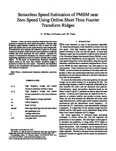
A. Simulations of the Three Methods The simulation plots for the least-squares case are given in Fig. 1. The full load torque τ L = 2000 Nm is assumed. The sampling period for the speed estimator was 0.1 millisec and the forgetting factor λ was 0.99. The left-hand plot is the speed and its reference, with the rotor resistance in the motor model changed from its nominal value of RR = 0.187Ω to RR = 0.3Ω. This results in a 5% speed tracking error. The plot of the right-hand side is under the same conditions (with the rotor resistance returned to its nominal value RR = 0.187Ω), except that the stator resistance in the motor model was changed from its nominal value of RS = 0.262Ω to RS = 0.5Ω (about 100% increase, possibly due to ohmic heating). The deterioration in performance is quite pronounced. This simulation shows the significant impact of parameter variations and the need for joint estimation of the speed and of the motor parameters. Fig. 2 shows the simulation results for the nonlinear scheme given in [31]. It was found that the load torque had to be reduced to τ L = 1700 Nm in order to achieve tracking with the nominal parameters. The plot on the lefthand side shows the speed ω and speed reference ω ref , assuming nominal parameters in both the estimator and the controller (perfect parameter match). The right-hand side

Speed (rad/s)

150

100

50

100

50

0

0

0

2

4

6

8 10 12 14 16

0

2

4

6

8 10 12 14 16

Time (s)

Time (s)

Fig. 1. Speed and speed reference (least-squares scheme). Left: RR = 0.187Ω. Right: RR = 0.3Ω. 180 160

0

140

-200

120

-400

Speed (rad/s)

Speed (rad/s)

The sensorless control problem may be stated as follows (a) achieve vector control of the induction motor for speed and/or torque tracking; (b) be robust to parameter uncertainty; (c) handle full rated load-torque on the motor at start-up; (d) achieve rated speed of the motor in steadystate. These conditions are typically required of a fieldoriented control system with a sensor. To demonstrate the capabilities and limitations of the existing approaches, simulation models of the above senR sorless control schemes were developed using Simnon° . The motor under consideration was a 500 Hp, 3-phase induction motor (see [15], p.190), with the motor parameters np = 2, nph = 3, RS = .262Ω, RR = .187Ω, J = 11.06 kg-m2 , LS = .1465 H, LR = .1465 H, M = .143 H, Vline−line max = 2300 Volts. The stator leakage inductance is lS = LS − M = .0035 H and the rotor leakage inductance is lR = LR − M = .0035 H. The synchronous speed is 2π(60/np ) = 188 rad/sec, giving a rated speed of 180 rad/sec at 3% rated slip. The base speed is 80 rad/sec (i.e., the speed at which field weakening is started) and the rated load torque is τ L = 2000 Nm. In all the simulations, the machine flux was allowed to build up to its nominal value ψ do = M id0 , with id0 = 50 Amps. The trajectory and load torque τ L were applied at t = 4 seconds. The plots show that the motor speed actually becomes negative at first due to the application of the load torque at t = 4 seconds. This effect would also be seen using a field-oriented controller with a shaft sensor, and could be lessened by estimating the load torque and feed-forwarding the estimate to the controller.

Speed (rad/s)

150

100 80 60

-600 -800 -1000

40

-1200

20

-1400

0

-1600 0

2

4

6

8

10

Time (s)

12

14

16

0

2

4

6

8

10

12

14

16

Time (s)

Fig. 2. Speed and speed reference (nonlinear scheme). Left: RS = 0.262Ω. Right: RS = 0.29Ω.

shows the speed plots with the stator resistance in the motor model changed from its nominal value of RS = 0.262Ω to RS = 0.29Ω (a change of only 10%). The system could not handle this small variation in the stator resistance. Again, a significant sensitivity to parameter uncertainty is observed with this method. In view of these observations, the adaptive sensorless scheme proposed in [22], designed to be insensitive to the value of the stator resistance RS , would seem quite attractive. It does require knowledge of the rotor time constant TR (RR ), but so does the standard field-oriented controller with a position sensor. However, in our simulations, we were unable to get this sensorless scheme to work unless the load torque was very low (τ L = 400 Nm or 20% of rated torque) and the motor was not allowed to decelerate. The plots shown in Fig. 3 give a comparison with a load of τ L = 400 Nm on the left and with a load of τ L = 500 Nm on the right. Interestingly, it was found that the estimator itself worked fine if it was not used for feedback control, that is, if the true speed was fed back rather than its estimate. This observation indicates that, in addition to addressing the joint speed/parameter estimation problem, any practical sensorless control methods should also consider the joint control/estimation problem. We simulated the other sensorless scheme given in [22] (described above), which is a modification of the scheme presented by Shauder [25]. In our simulations, this scheme

3080

6

100

160

80

140

60

120

Speed (rad/s)

Speed (rad/s)

180

100 80 60

[7]

40

[8]

20 0 -20

40

-40

20

-60

[9] [10]

-80

0 0 1 2

3 4

5 6 7

8 9

0

1

2

3

4

5

6

7

[11]

Time (s)

Time (s)

Fig. 3. Speed and speed reference (adaptive sensorless scheme). Left: τ L = 400 Nm. Right: τ L = 500 Nm.

worked for deceleration, but still could only accommodate small load torques (τ L < 500 Nm) even under nominal conditions (no parameter uncertainty). We also simulated the original adaptive approach of Shauder [25], and it was able to handle a load τ L = 1700 Nm, a variation in the stator resistance from 0.262Ω to 0.4 (50%), but only a variation in the rotor resistance of 15% (from 0.187Ω to 0.2Ω).

In summary, the above simulations indicate the difficulty in trying to do sensorless control and perhaps the need to not limit oneself to anyone particular algorithm. Algorithms should provide sensorless control under full load (to avoid over sizing the motor) while allowing for variations in stator resistance and in rotor time constant. A satisfactory solution may be obtained through the combination of above techniques. For example, the least-squares approach could be modified to estimate the stator resistance RS and the rotor time constant TR in addition to the speed. In essence, this approach would be the combination of the parameter identification in [26], together with the method of Verghese et al [19] [28] [29]. Another idea would be to combine the method of [22], which is insensitive to RS , with another method; for example, the speed estimate of [22] would not be fed back, but instead would be used to calibrate the errors in another estimator that is sensitive to RS . References

[2] [3] [4] [5] [6]

[13] [14]

[15] [16] [17]

III. Conclusions

[1]

[12]

[18]

[19]

[20] [21] [22]

[23] [24] [25]

[26]

Baader, U. and M.Depenbrock, “Direct Self Control (DSC) of Inverter-Fed Induction Machine A Basis for Speed Control without Speed Measurement,” IEEE Trans. on Industry Applications, vol. 28, no. 3, May/June 1992. Boldea, I., and S.A. Nasar, Electric Drives , CRC Press, Boca Raton, FL, 1999. Bodson, M. and J. Chiasson, “Differential-Geometric Methods for Control of Electric Motors”, International Journal of Robust and Nonlinear Control, vol. 8, pp. 923-954, 1998. Bodson, M., and J. Groszkiewicz, “Multivariable Adaptive Algorithms for Reconfigurable Flight Control,” IEEE Trans. on Control Systems Technology, vol. 5, no. 2, pp. 217-229, 1997. Bodson, M., J. Chiasson and R. Novotnak, “High performance nonlinear control of an induction motor via input-output linearization,” IEEE Control Systems, pp. 25-33, August 1994. Bodson, M., J. Chiasson and R. Novotnak, “Nonlinear speed observer for high-performance induction motor control,” IEEE Trans. on Industr. Electronics, vol. 42, no. 4, pp. 337-343, 1995.

[27] [28]

[29] [30] [31]

3081

Bodson, M., J. Chiasson and R. Novotnak, “A systematic approach to selecting flux references for torque maximization in induction motors,” IEEE Trans. on Control Systems Technology, vol. 3, no. 4, pp. 388-397, December 1995. Chiasson, J., “Dynamic Feedback Linearization of the Induction Motor,” IEEE Trans. on Automatic Control, vol. 38, no. 10, pp. 1588-1594, October 1993. Chiasson, J., “Differential-Geometric Techniques for Control of a Series DC Motor,” IEEE Trans. on Control Systems Technology, vol. 2, no. 1, pp. 35-42, March 1994. Chiasson, J., “Nonlinear Controllers for an Induction Motor”, Control Engineering Practice, vol. 4, no. 7, p. 977-990, 1996. Chiasson, J., “A New Approach to Dynamic Feedback Linearization of the Induction Motor,” IEEE Trans. on Automatic Control, vol. 43, no. 3, pp. 391-397, March 1998. Feemster, M., P. Aquino, D.M. Dawson and D. Haste, “Sensorless Rotor Velocity Tracking Control for Induction Motors,” IEEE Trans. on Control Systems Technology, pp. 645-653, vol. 4, No. 4, July, 2001. Ha, I.-J. and S.-H. Lee, “An On-Line Identification Method for Both Stator and Rotor Resistances of Induction Motors without Rotational Transducers”, ISIE ’96, Warsaw Poland, June 1996. Jönsson, R. and W. Leonhard, “Control of an Induction Motor without a Mechanical Sensor, based on the Principle of Natural Field Orientation (NFO),” Proc. of the International Power Electronics Conference, April 1995, Yokohama, Japan. Krause, P.C., Analysis of Electric Machinery, McGraw-Hill, 1986. Leonard, W., Control of Electrical Drives, New York SpringerVerlag, 1985. Leonard, W., Control of Electrical Drives, Second Edition, New York Springer-Verlag, 1997. Marino, R., S. Peresada, and P. Tomei, “Global Adaptive Output Feedback Control of Induction Motors with Uncertain Rotor Resistance,” IEEE Trans. on Automatic Control, vol. 44, no. 5, pp. 967-983, May 1999. Minami, K., M. Vélez-Reyes, D. Elten, G.C. Verghese and D. Filbert, “Multi-stage speed and parameter estimation for induction machines,” IEEE Power Electronics Specialist’s Conference, Boston MA, June 1991. Mueller, K., “Efficient TR Estimation in Field Coordinates for Induction Motors,” IEEE International Symposium on Industrial Electronics, Bled, Slovenia, July 12-16, 1999. Novotnak, R.T., J. Chiasson and M. Bodson, “High Performance Control of an Induction Motor with Saturation,” IEEE Trans. on Control Systems Technology, vol. 7, no. 3, pp. 315-327, 1999. Peng, F. Z. and T. Fukao, “Robust Speed Identification of for Speed-Sensorless vector control of induction motors”, IEEE Trans. on Industry Applications, vol. 30, no. 5, pp. 1234-1240, September/October 1994. Rajashekara, K., A. Kawamura, K. Matsuse, Editors, Sensorless Control of AC Motor Drives - Speed and Position Sensorless Operation, IEEE Press, 1996. Sastry, S. and M. Bodson, Adaptive Control Stability, Convergence, and Robustness, Prentice Hall, 1989. Shauder, C., “Adaptive speed identification scheme for vector control of induction motors without rotational transducers,” IEEE Trans. on Industry Applications, vol. 28, no. 5, pp. 10541061, September/October 1992. Stephan, J., M. Bodson, and J. Chiasson, “Real-time estimation of induction motor parameters,” IEEE Trans. on Industry Applications, vol. 30, no. 3, pp. 746-759, May/June 1994. Vas, P., Sensorless Vector and Direct Torque Control, Oxford Press, 1998. Vélez-Reyes, M. and G.C. Verghese, “Decomposed algorithms for speed and parameter estimation in induction machines,” IFAC Symposium on Nonlinear Control System Design, Bordeaux France, 1992. Vélez-Reyes, M., K. Minami, G. C. Verghese, “Recursive Speed and Parameter Estimation for Induction Machines,” IEEE Industry Applications Society Meeting, San Diego, 1989. Verl, A., and M. Bodson, “Torque Maximization for Permanent Magnet Synchronous Motors,” IEEE Trans. on Control Systems Technology, vol. 6, no. 6, pp. 740-745, 1998. Yoo, H.-S. and I.-J. Ha, “A Polar Coordinate-Oriented Method of Identifying Rotor Flux and Speed of Induction Motors without Rotational Transducers,” IEEE Trans. on Control Systems Technology, vol. 4, no. 3, pp. 230-243, May 1996.