Separation-Resistant and Bias-Reduced Logistic Regression ...

JSS

Journal of Statistical Software April 2012, Volume 47, Code Snippet 2.

http://www.jstatsoft.org/

Separation-Resistant and Bias-Reduced Logistic Regression: STATISTICA Macro Kamil Fijorek

Andrzej Sokolowski

Cracow University of Economics

Cracow University of Economics

Abstract Logistic regression is one of the most popular techniques used to describe the relationship between a binary dependent variable and a set of independent variables. However, the application of logistic regression to small data sets is often hindered by the complete or quasicomplete separation. Under the separation scenario, results obtained via maximum likelihood should not be trusted, since at least one parameter estimate diverges to infinity. Firth’s approach to logistic regression is a theoretically sound procedure, which is guaranteed to arrive at finite estimates even in a separation case. Firth’s procedure was also proved to significantly reduce the small sample bias of maximum likelihood estimates. The main goal of the paper is to introduce the STATISTICA macro, which performs Firth-type logistic regression.

Keywords: logistic regression, complete separation, STATISTICA.

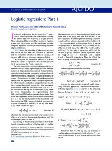
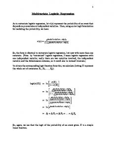
1. Introduction 1.1. Logistic regression model Logistic regression is a commonly used tool to describe the relationship between a binary outcome variable and a set of explanatory variables. It is routinely employed in many fields, e.g., medicine, social sciences, economics. The popularity of logistic regression stems mainly from its mathematical convenience and the relative ease of interpretation in terms of odds ratios (Hosmer and Lemeshow 2000; Long 1997; Greene 2003). Assume that the dependent variable yi ∈ {0, 1} is a Bernoulli distributed variable with success probability F (x> i θ), where F (◦) is the logistic distribution function, xi is a p-dimensional vector of explanatory variables and θ ∈ Rp is a p-dimensional parameter vector (i = 1, . . . , n). The most frequently used estimation method of θ is the maximum likelihood estimation

2

Separation-Resistant and Bias-Reduced Logistic Regression: STATISTICA Macro

(MLE). The MLE principle states that the estimate of θ is the value which maximizes the likelihood function (Hosmer and Lemeshow 2000). The likelihood function and its logarithm in case of logistic regression are given by the following equations: n Y

yi > 1−yi F (x> , i θ) [1 − F (xi θ)]

(1)

> yi ln F (x> i θ) + (1 − yi ) ln[1 − F (xi θ)].

(2)

L(θ) =

i=1

l(θ) =

n X i=1

In order to find the value of θ that maximizes L(θ), partial derivatives of a log-likelihood function with respect to θ are calculated: n X U (θ) = [yi − F (x> i θ)]xi .

(3)

i=1

ˆ The solution to score equations U (θ) = 0 gives the ML estimate of θ, i.e., θ. In most cases, there is no analytical solution to score equations. Consequently, numerical ˆ With starting value θ(1) , the maximum likelihood estimate θˆ is methods are used to find θ. obtained iteratively: (r) , (4) θ(r+1) = θ(r) + Iθ−1 U θ (r) where the superscript (r) refers to the r-th iteration and Iθ denotes the Fisher information matrix evaluated at θ (Greene 2003): Iθ = −

n X ∂ 2 li (θ) i=1

∂θ∂θ>

=

n X

> F (x> θ) 1 − F (x θ) xi x> i i i .

(5)

i=1

The desirable properties of ML estimates such as: consistency, efficiency and normality, are based on the assumption that the sample size (n) approaches infinity. However in many real life situations the large sample assumption is not satisfied, and as a result, ML estimates should not be trusted. The bias of ML estimates in small samples can be substantial. Moreover, in small samples, there is a non-negligible probability of encountering the separation. From the geometrical point of view the separation occurs when there exists a hyperplane which separates successes and failures (complete separation), where the hyperplane itself may contain both successes and failures (quasicomplete separation). In that case, at least one parameter estimate diverges to infinity (Albert and Anderson 1984; Heinze and Schemper 2002). In practice, the separation phenomenon can be detected by tracking the magnitude of standard errors. The most common strategy to deal with separation is to remove any offending variable(s) from the model. However, this approach is seriously flawed since the omission of any important variable(s) is inappropriate.

1.2. Penalized maximum likelihood Firth (1992a,b, 1993) derived the procedure that guarantees finite estimates of logistic regression parameters in case of separation; it was also proven to significantly reduce the small

Journal of Statistical Software – Code Snippets

3

sample bias of maximum likelihood estimates, i.e., the first-order term is removed from the asymptotic bias of maximum likelihood estimates. The procedure originally developed by Firth (1993) was further researched and popularized by the work of Heinze and Schemper (2002), Heinze and Ploner (2004), and Heinze (2006). The basis of Firth’s approach is the idea that the bias in θˆ can be reduced by modifying the score equations. The modified equation has the following form: U ∗ (θ) =

n X 1 > yi − F (x> θ) + h − F (x θ) xi , i i i 2

(6)

i=1

1

1

where hi is the i-th diagonal element of the H matrix H = W 2 X(X > W X)−1 X > W 2 is a n × p data matrix and W is a n × n diagonal matrix with the i-th diagonal element > > F (xi θ) 1 − F (xi θ) . The modification to score equations can alternatively be introduced by penalizing the original likelihood function: 1 (7) L∗ (θ) = L(θ)|Iθ | 2 . It is interesting that Firth’s approach to logistic regression is identical to Bayesian logistic regression with noninformative Jeffreys prior. Penalized maximum likelihood estimates (PMLE) can be found with the use of the numerical (r) routine described above with U θ term replaced by U ∗ θ(r) .

1.3. Statistical inference Estimation of standard errors can be based on the roots of the diagonal elements of I ˆ−1 , which θ 2 ∗ −1 ∂ l (θ) −1 ∗ = − ∂θ∂θ> is a first-order approximation to Iθ (Firth 1992a,b, 1993; Bull, Mak, and Greenwood 2002). According to the simulation study performed by the authors (results not shown), there is no clear advantage of using Iθ∗ −1 in place of Iθ−1 with respect to the number of iterations needed for convergence and the coverage of a Wald confidence interval. However, more extensive study regarding this subject would be useful. Appropriate simulation studies can be greatly facilitated by the recent work of (Chen, Ibrahim, and Kim 2008) from which the closed form of Iθ∗ −1 can be easily obtained. Given the estimate of the covariance matrix I ˆ−1 , one can compute Wald confidence intervals θ and p values based on the normal approximation to the distribution of the PML estimates. The (1 − α)% Wald confidence interval for θj , (j = 1, . . . , p) is given by: q q θˆj − z1− α2 (I ˆ−1 )j ; θˆj + z1− α2 (I ˆ−1 )j , (8) θ

θ

ˆ z1− α is the 1 − α quantile of the standard where θˆj is the PML estimate of j-th element of θ, 2 2 −1 normal distribution function and (I ˆ )j is a j-th diagonal element of I ˆ−1 . θ

θ

It should be noted, however, that in small samples the coverage probability of the Wald confidence interval may deviate from its nominal value. This behavior was observed in simulation studies performed by (Heinze 1999), it was also shown there that profile likelihood confidence intervals are superior to Wald intervals. Simulation studies performed by the authors (results not shown) led to similar conclusions.

4

Separation-Resistant and Bias-Reduced Logistic Regression: STATISTICA Macro

2. STATISTICA macro The STATISTICA data analysis software system (StatSoft, Inc. 2010) offers a user-friendly module for maximum likelihood estimation of logistic regression coefficients. As was mentioned above, the maximum likelihood estimation is not resistant to the separation problem and, generally speaking, is not suitable for small datasets. This was the main motivation for the implementation of a STATISTICA macro performing Firth-type logistic regression. The presented macro was written in SVB (the Visual Basic programming environment integrated with STATISTICA) in STATISTICA 9.1. SVB is similar to Microsoft Visual Basic 6, as well as the Visual Basic language available in Microsoft Excel. SVB includes a comprehensive library of optimized matrix procedures. The employment of built-in matrix functions resulted in a more readable macro code. The macro code was partly based on a source code of the R (R Development Core Team 2012) package logistf (Heinze and Ploner 2004; Ploner, Dunkler, Southworth, and Heinze 2010). An alternative R implementation offering similar functionality is available in the package brglm (Kosmidis 2011), based on the recent work of Kosmidis and Firth (2009).

2.1. Starting a macro Launch STATISTICA and open a dataset of interest. Open the macro file named SR_BR_LR.svb (separation-resistant bias-reduced logistic regression), available along with this manuscript. Press the F5 keyboard button or left-click the Run Macro button on the Macro toolbar (see Figure 1). The variable selection window should appear. The list of variables available for analysis is automatically loaded from the active workbook. Select appropriate variables and press the OK button. After a short time, an output window should appear.

If one plans to use the macro frequently, then a different approach should be taken, i.e., the macro should be installed. This process creates a button which automatically starts the macro without the need to manually reopen the macro file every time STATISTICA is restarted. To install the macro file:

Figure 1: The localization of the Run Macro button on the Macro toolbar.


Figure 2: The localization of the Customize button.

Figure 3: The localization of the Commands list.

Figure 4: The effect of the macro installation.

5

6

Separation-Resistant and Bias-Reduced Logistic Regression: STATISTICA Macro Launch STATISTICA. Open the macro file named SR_BR_LR.svb. Right-click on any toolbar and select the Customize (see Figure 2). Go to the Command/Macros tab, select Macros from the Categories list, and from the Commands list, drag the macro name (i.e., SR_BR_LR) from its original position to the main toolbar (see Figure 3 and 4). Press the newly created button to start the macro.

2.2. Generated output The output generated by the macro consists of a workbook with three spreadsheets. The first spreadsheet holds the original values of the dependent variable along with estimated probabilities of a success. The second spreadsheet holds the estimate of the covariance matrix, i.e., I ˆ−1 . The third spreadsheet is of the most importance as it shows the following: θ

The number of iterations needed for convergence. The value of log-likelihood at last iteration. Parameter estimates. Standard errors (SE) of parameter estimates. 95% Wald confidence intervals for parameters. Odds ratios for a unit increase in the independent variables. 95% Wald confidence intervals for odds ratios. P values for a hypothesis test that a given parameter is equal to zero.

In the current version of the macro, profile penalized likelihood confidence intervals are not implemented. They are, however, planned for future release.

3. Examples 3.1. Toy example The toy dataset was constructed to demonstrate the case of the infiniteness of ML estimates in logistic regression. The data matrix X in the first column contains 1s and the only explanatory variable assumes 10 equidistant values from 1 to 10. The first 5 values of dependent variable (y) are failures (0) and the last 5 are successes (1). One can clearly see the complete separation,


7

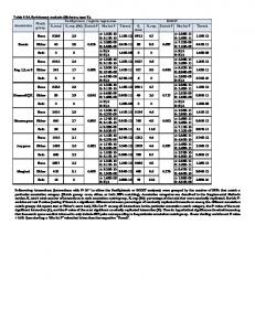
Figure 5: STATISTICA macro output – toy dataset. i.e., all cases are failures where the value of the explanatory variable is less than 6 and all cases are successes where the value of the explanatory variable is greater than or equal to 6. > 1 1 1 1 1 1 1 1 1 1 X = 1 2 3 4 5 6 7 8 9 10 > y = 0 0 0 0 0 1 1 1 1 1 To estimate the logistic regression model on this dataset, we used both the package logistf and our macro. Below we show the necessary commands to create the toy dataset, estimate the model and visualize the results. Figure 6 presents the dataset along with the fitted logistic function. Figure 5 shows a screen capture of the output of our macro. The estimation results of both the package logistf and our macro are in very close agreement. R> R> R> R> R>

library("logistf") X R> R> R> R> R>

C1 + R>

data("Banknotes", package = "ncomplete") bank