Simple algorithm for recurrent neural networks that ... - Semantic Scholar

Simple algorithm for recurrent neural networks that can learn sequence completion Istv´an Szita and Andr´as L˝orincz Department of Information Systems E¨otv¨os Lor´and University Budapest, H-1117 Hungary E-mail: [email protected]

Abstract— We can memorize long sequences like melodies or poems and it is intriguing to develop efficient connectionist representations for this problem. Recurrent neural networks have been proved to offer a reasonable approach here. We start from a few axiomatic assumptions and provide a simple mathematical framework that encapsulates the problem. A gradient-descent based algorithm is derived in this framework. Demonstrations on a benchmark problem show the applicability of our approach.

I. I NTRODUCTION A. Motivation In this paper we try to build a simple mathematical model which is able to reproduce certain properties of human memory. Humans can to learn long sequences of data (for example, melodies, lyrics etc.) just by observing them a couple of times. One interesting property of this kind of learning is that it has directional bias: learning facilitates recall in forward direction. Another property of this sort of memory is robustness: we are able to recognize portions which are covered by noise. We believe that this kind of memory works in an essentially different way than databases or tables do. Our aim is to give a feasible model for sequence learning, making only a few fundamental assumptions. These assumptions are: (1) the algorithm should be simple and connectionist (2) observing a portion of a known sequence, the algorithm should be able to continue the sequence regardless of the position of this portion, and (3) the solution should be noise tolerant. We have chosen recurrent neural networks (RNNs) to accomplish the task, because of their flexibility and ability to represent long time series. The suitability of the RNN approach has been suggested by many researchers, including [1], [2], where it was used to predict chaotic time series, or financial data [3], [4]. In [5], RNN was used for signal processing, whereas [6] aimed natural language processing by means of RNN. B. Previous Work The amount of publications on learning, representing and retrieving dynamic data sequences in neural systems is surprisingly small. One attempt is made by Barreto and Ara´ujo [7], [8]. They train a neural network to replay sequences exactly as they appeared originally. However, in their approach

temporal ordering is essentially hand-wired, and the usability of local context neurons to resolve ambiguities also seems limited. Another approach is the fractal prediction machine of Tiˇno and Dorffner [9], which is able to learn the longterm characteristics of a time series. Their solution is based on iterated function systems, which is in close relationship with neural networks, but the connectionist algorithm remains to be developed. An approach similar but not identical to sequence learning is multi-step prediction. Bon´e and Crucianu [10] give an excellent review on existing multi-step prediction methods. These are mostly iterated versions of one-step predictors. There exists a great variety of algorithms for learning time series prediction using RNNs. Recurrent backpropagation and backpropagation through time (BPTT) [11], [12], [13], real-time recurrent learning (RTRL) [14], [15], or extended Kalman-filter (EKF) based training [16], [17] are such examples. For a review on these algorithms and a unifying framework, see [18]. However, one-step prediction methods must be handled with caution: according to Bon´e and Crucianu [10], in the general case, their performance may be poor when they are used iteratively for multi-step ahead prediction. Extensions that take into account long-term dependencies could be helpful: Hochreiter and Schmidhuber introduced their long short-time memory (LSTM) method, which is capable to learn dependencies on an extremely large scale [19]. Despite this, LSTM is not always suitable for multi-step prediction: Gers et al. [20] have shown that despite its attractive capabilities, LSTM can fail even on simple problems. An approach similar to ours is the method of Bakker et al. [21]. They have successfully trained neural networks to learn chaotic time series, using “error propagation” augmented with principal component analysis and monitoring of chaotic invariants. However, the error propagation method takes multistep prediction errors into account only implicitly, thus improvement of performance cannot be guaranteed theoretically. Methods that inject finite state automata (FSA) into neural networks should be mentioned: these are promising tools for processing temporal data, with rich literature. However, that subject is out of the scope of this paper.

C. Our Approach We formulate an appropriate sum-of-squares error function, that directly takes into account the sequence replay error. Thus, training decreases not only the one-step prediction error, but multi-step errors as well. Of course, this comes at a price: the error function becomes more complex, so a backpropagation-like algorithm cannot minimize it efficiently. However, we show that by exploiting the special structure of the error function, it is still possible to construct a gradientdescent-based algorithm with good performance. D. Paper Outline First, we shall formalize the sequence replay problem and the proposed RNN architecture. Next, a simple least-squares method for RNN training is described and some analysis on its performance is provided. Then in Section IV we test the algorithm on some simple benchmark problems. Finally, we summarize and discuss our results. II. D EFINITIONS AND BASIC CONCEPTS We investigate the following simple model of sequence replay: Assume a time series, which is a sequence of Rm vectors. The RNN architecture has to learn q such sequences, in the sense that if the first several elements of a sequence are shown to the network, it is able to replay the remainder. For the sake of simplicity we consider batch learning only, that is, we assume that all the sequences are known in advance. To keep the formalism simple, we shall consider the slightly more complex problem where there is only one T step sequence to be learnt, but we may start to give inputs from an arbitrary point of the sequence, and the network has to continue replaying from that point on. B. The network architecture The network that is trained to accomplish this task will be an Elman-type fully recurrent neural network specified below. Let the input be m-dimensional, and denote its value at time t by xt . The network has n neurons, so its state at time t is an n-dimensional vector ut (n > m). The input activities are fed into the network by the input weight matrix G ∈ Rn×m , the recurrent weights are given by weight matrix F ∈ Rn×n , and the bias weights by b ∈ Rn . To simplify notation, we incorporate the bias b into the input weights using the standard technique: the input is augmented by an additional component which is clamped to +1 and has input weights Gm+1 = b. There are no specific output neurons in our network, simply the states of the first m neurons are considered as outputs. This can be formalized by an output weight matrix H ∈ Rm×n that is a projection to the first m coordinates. Because the network will be used for input prediction, we denote the output at time t by x ˆt+1 . So the dynamics of the network can be given by the following equations = =

σ(F ut + G[xt ; 1]), Hut+1 ,

and we assume that the iteration starts from u1 = 0.1 Later on, it will be useful to define the policy corresponding to a weight matrix F0 , denoted by πF0 , which describes the effect of F0 on a state vector ut : πF0 (ut ) := σ(F0 ut + G[xt ; 1]).

(4)

Note the implicit dependence on t. With this notation, the dynamics (1)–(2) can be written as ut+1 x ˆt+1

= =

πF (ut ), Hut+1 ,

(5) (6)

III. C ONSTRUCTION OF THE A LGORITHM

A. Problem specification

ut+1 x ˆt+1

where σ is either the identity (linear RNNs) or some nonlinear squashing function like tanh(x) or the saturated linear squashing function  if −1 < x < 1;  x, −1, if x ≤ −1; σ(x) = , (3)  +1, if x ≥ 1.

(1) (2)

We follow a traditional way of constructing learning algorithms: we define an error function that characterizes the inaccuracy of the weight matrices learned, and then apply a gradient-descent-based method for minimizing it. To keep the derivation as simple as possible, we assume that the weight matrix G is known in advance, and only F is tuned, although the same technique could be used to tune both F and G. A. The basic algorithm Let UF be the state sequence generated by eq. (5), i.e. UF := {ut | t = 1, . . . , T ; u1 = 0, ut = πF (ut−1 )} . (7) In general, we may consider state sequences that are not generated by a single weight matrix: let U = {ut | t = 1, . . . , T }

(8)

be an arbitrary state sequence. Using some fixed weight matrix F for prediction, the k-step prediction error of a single state ut0 is H(πF )k (ut ) − xt+k . (9) Using this, we can define a measure of prediction error for an arbitrary state sequence U as the sum of squared norms of all k-step prediction errors with k ≤ K: J(U, F ) :=

T min(K,T X X −t) ° ° °H(πF )k (ut ) − xt+k °2 . t=1

(10)

k=1

Unfortunately, this error function is a high-degree polynomial of F even for moderate values of K and for linear RNNs, and matters become even more complicated if σ(.) is a nonlinear squashing function. In turn, gradient-descent methods are not particularly well-suited: the error function 1 There are several methods for setting the initial state appropriately. In this paper we do not deal with this question. The interested reader is referred to [17] where an excellent overview is provided on this subject.

may have many extremal points and the global optimum can have a vanishingly small basin of attraction. Our approach is similar to ”coordinate descent”, the variant of gradient descent, where in each iteration a single (or a few) parameter is minimized, keeping all the other parameters fixed. If each parameter is chosen equally often, coordinate descent has the same convergence properties as gradient descent. In our case, we consider every instance of F as a separate parameter. At a minimization step, in each term we keep all but one instance of F fixed, and allow to vary only the last occurrence. In other words, we minimize the following function with respect to F :

Proof: For K ≥ T and F = F0 + ∆F the cost function takes the form JF0 (U, F0 + ∆F ) = T T −t X X ° ° °H(πF )k−1 πF +∆F (ut ) − xt+k °2 = 0 0 =

t=1 k=1 T T −t X X

(13)

° ° °H(πF0 )k−1 πF0 +∆F (πF0 )t (u0 ) − xt+k °2 .

t=1 k=1

Let V (F ) :=

T X ° ° °H(πF )j (u0 ) − xj °2 .

(14)

j=1

JF0 (U, F ) :=

(11)

T min(K,T X X −t) ° ° °H(πF0 )k−1 πF (ut ) − xt+k °2 . t=1

k=1

This error function is much easier to minimize: for all strictly increasing squashing function σ it has a unique minimum. Moreover, for linear RNNs, it is a quadratic function of F , so the minimum can be computed in a closed form. Recall that U was originally the state sequence generated by F , so in order to keep the simplicity of the minimization, we have to fix its value to UF0 as well. In order to keep the structure of the problem simple, in the following steps we do not vary the places of F s to be minimized, but we simply move F0 towards F by a small amount: F0 := F0 + αt (F − F0 ),

(12)

and iterate these steps. The obtained algorithm is summarized in Figure 1. (1) F0 ;

Initialize i := 1 repeat U(i) := UF (i) 0

F (i) := arg minF JF (i) (U(i) , F ) (i+1)

(i)

0

(i)

F0 := F0 + αt (F (i) − F0 ) i := i + 1 (i) until F0 converges Fig. 1.

Schematic description of the basic algorithm

B. Analysis The proposed algorithm is gradient-descent-based so, at most, convergence to some local minimum can be proved. A somewhat weaker statement shall be proved here: Theorem 3.1: Let F ∗ be an optimal weight matrix. If the iteration is started from a small enough neighborhood of F ∗ , and the learning rates are sufficiently small, the algorithm converges to F ∗ , if K ≥ T .

Notice that in JF0 (U, F0 + ∆F ) and V (F0 + ∆F ) the terms that are at most linear in ∆F are identical. This means that, firstly, a minimum of J is also a minimum of V , and secondly, for small enough ∆F , their gradients are essentially the same, because the second- and higher order terms can be neglected. Therefore, in a small neighborhood of F ∗ , our algorithm using J is equivalent to gradient descent on V , which converges to F ∗ if the assumptions on the learning rate αt are satisfied. C. Refined version of the algorithm Equation (12) for the tuning of F0 is highly nonlinear because all instances of the weight matrix F0 are changed simultaneously. That is, the above algorithm behaves very much like gradient descent, and most importantly, the optimum may have a relatively small basin of attraction. Therefore, more care seems necessary in the tuning of the weight matrices. We proceed by relaxing the conditions on the state sequence (i+1) U(i) . Instead of requiring ut = (πF0 )t (u0 ) for each t, we only require that (i+1)

ut

(i)

= πF0 (ut−1 ).

(15)

This relaxation has the advantage that the changes of F0 are not global but only take place locally, one step at a time. Note that in general it will not hold that U is a state sequence UF generated by some weight matrix F . This statement holds only (i) in the limit when F0 has converged. We will write U(i+1) = πF0 U(i) as a shorthand for Eq. (15). Furthermore, we add a regularization term X C· Fij2

(16)

(17)

ij

to our cost function to avoid degeneration. Note that this corresponds to applying a Gaussian prior to the weights [18]. The modified algorithm is summarized in Fig. 2. In the small neighborhood of an optimal weight matrix F ∗ , the behavior of the modified algorithm is essentially identical to the basic algorithm, hence the result on local convergence still holds. The main difference is in the global behavior: the modified U-update is can help the algorithm escape local minima. This expectation will be confirmed experimentally in the next section.

(1)

Initialize F0 ; U(1) = UF (1) ; i := 1 0 repeat F (i) := arg minF JF (i) (U(i) , F ) (i+1)

(i)

0

(i)

F0 := F0 + αt (F (i) − F0 ) (i+1) U := πF (i) U(i) 0 i := i + 1 (i) until F0 converges Schematic description of the refined algorithm

IV. E XPERIMENTS During the experiments we have used the refined version of our algorithm with saturated linear activation function. For computing the arg min, we approximate this by the identity function σ(x) = x, in which case JF0 (U, F ) is a quadratic function of F , and the minimum can be computed in closed form. For training the networks, we used K = 3, regularization coefficient C = 1 and a constant learning rate α = 0.1. The network had a single input neuron, the number of total neurons varied from 4 to 20. The input matrix G was chosen at random with all entries between 0 and 1. The Mackey-Glass delay-differential equation x(t) ˙ =

ax(t − τ ) − bx(t) 1 + xc (t − τ )

(18)

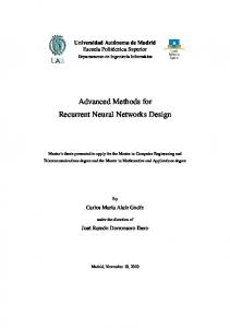
was first described in [22], and has become a standard benchmark problem with parameters a = 0.2, b = 0.1, c = 10, τ = 17 (for τ > 16.8 the series becomes chaotic), and a sampling rate of 6 s. We generated 200 data points for training, and further 200 for testing. Data were scaled to the interval [−1; 1]. After several iterations, the replay capabilities of the learned weight matrix were tested: the network was reset to u1 = 0, then it was allowed to observe N1 consecutive inputs from the time series, starting from some randomly chosen t0 . After the observation, it had to reproduce the following N2 values of the time series without external input. The effect of training is demonstrated in Fig. 3. According to Fig. 3, a network trained by the algorithm may be able to replay sequences. However, this single example proves very little and further questions need to be answered: is the network always able to learn the time series? If so, to what extent? What is the dependence on the number of neurons? The next sequence of test runs aim to provide answers to these questions. We have trained networks with n neurons (n = 4...20) for 100 episodes, and tested them. Because the input matrix G (which is chosen at random) affects performance, we have performed 20 parallel runs for each n. Testing was done by choosing a random starting time t0 , after which the network was allowed to observe the next N1 = 10 inputs. The network then had to replay the consecutive N2 = 10 input values, and

Fig. 3. Sequence replay. Number of neurons: 12, t0 chosen at random. Solid black line: the Mackey-Glass time series. Gray lines: network performance after various amounts of training: 5 episodes (dotted gray), 15 episodes (dashed gray), 50 episodes (solid gray). Vertical line: end of observation and beginning of unguided replay. N1 = N2 = 20 time steps.

0.25

error

Fig. 2.

0.2

0.15 0.1 5

10 15 Number of neurons

20

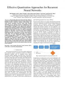
Fig. 4. Dependence of sequence replay error on network size. See text for details. Each data point is the average of 20 test runs. Gray area denotes ±standard deviation.

the mean squared error et =

1 N2

t0 +N 1 +N2 X

|ˆ xt − xt |2

(19)

t=t0 +N1 +1

was recorded. For each trained network we repeated this test 30 times with different t0 values, and averaged the results, which are summarized in Fig. 4. The test runs show that for this problem, network size has little impact on the average performance: 6 neurons are able to learn the task almost as well as 20 neurons do. The great difference is in their reliability: the more neurons a network has, the smaller the probability that an unfortunate choice of G prevents it from learning. We have repeated the same experiment so that the input data used for training and testing are chosen from different sections of the Mackey-Glass time series. The results, within error bounds, are identical to Fig. 4, thus the extra figure is omitted. As a final test in this domain, we examined the effect of the observation length N1 on the sequence replay error. To this

0.4

B. Possible areas of application

error

0.3

0.2

0.1

0 0

5 10 15 Number of observations

20

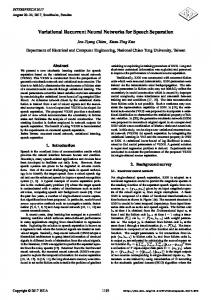
Fig. 5. Dependence of sequence replay error on observation length. See text for details.

end, we fixed a network with 12 neurons arbitrarily and trained it for 100 episodes. The replay length was fixed to N2 = 10, and the method of calculating the error was the same as above. The results, that are shown in Fig. 5, are not unexpected: replay error drops rapidly as more inputs become observable, until about N1 = 10. Afterwards, further observations are essentially useless, because the network is already adjusted as much as it could be.

The sequence completion capabilities of our algorithm can be an important tool in breaking the curse of dimensionality of sequential decision making: theoretically, it is possible that the agent makes decisions only every N th step, and in the intervals between them, interpolation is done by the network. In this case, a form of time compression is achieved: the agent can make decisions on a larger scale. Such extension would fit our event-learning formalism [23], [24]. Another important area of application is the prediction of time series (e.g. the analysis of financial data), for which our algorithm also provides a simple method (although it may not be as efficient as algorithms specifically designed for this task). Besides its simplicity, it has the great advantage that it is able to handle missing data. ACKNOWLEDGEMENT The authors would like to thank Zolt´an Szab´o for his helpful comments. This material is based upon work supported by the European Office of Aerospace Research and Development, Air Force Office of Scientific Research, Air Force Research Laboratory, under Contract No. FA8655-03-1-3036. Any opinions, findings and conclusions or recommendations expressed in this material are those of the author(s) and do not necessarily reflect the views of the European Office of Aerospace Research and Development, Air Force Office of Scientific Research, Air Force Research Laboratory.

V. D ISCUSSION In this paper we presented a neural network algorithm that is able to memorize general [−1, 1]m -valued data sequences by minimizing a least-squares error function that takes into account multi-step prediction error. The trained networks are able to replay the learned sequences, and complete them after showing a portion of them. We have demonstrated the capabilities of our algorithm on a simple one-dimensional time series. A. Extensions Throughout this paper we assumed that there is only one sequence to be learned. However, it is quite simple to apply the algorithm to the multiple sequence case, either by concatenating them (with delimiter-inputs if necessary) or by modifying the error function J by summing over sequences as well. In real-life applications it is inevitable to handle missing or sparse input data, which is an active field of research. Our method can handle missing data with ease: if no input signal arrives, it can be automatically substituted by the input replayed by the network. Essentially the same was done while the replay capabilities of the network were tested: after observing the beginning of the input sequence, the replayed part can be considered as missing input. A serious drawback of the method described here is that it works in batch mode. However, the algorithm is gradientdescent based, and the corresponding online version is currently under study.

R EFERENCES [1] J. Kuo, J. Principe, and B. deVries, “Prediction of chaotic time series using recurrent neural networks,” in Proc. 1992 IEEE Workshop of Neural Networks in Signal Processing, 1992, pp. 436–443. [Online]. Available: citeseer.nj.nec.com/448496.html [2] R. Bon´e, M. Assaad, and M. Crucianu, “Boosting recurrent neural networks for time series prediction,” in International Conference in Artificial Neural Nets and Genetic Algorithms, D. Peearson, N. Steele, and R. Albrecht, Eds. Springer Computer Science, April 2003, pp. 18–22. [3] P. Tino, C. Schittenkopf, and G. Dorffner, “Financial volatility trading using recurrent neural networks,” IEEE-NN, vol. 12, pp. 865–874, July 2001. [Online]. Available: citeseer.nj.nec.com/506945.html [4] C. Giles, S. Lawrence, and A. Tsoi, “Noisy time series prediction using a recurrent neural network and grammatical inference,” Machine Learning, vol. 44, no. 1/2, pp. 161–183, July/August 2001. [Online]. Available: citeseer.nj.nec.com/giles01noisy.html [5] O. Nerrand, P. Roussel-Ragot, L. Personnaz, G. Dreyfus, and S. Marcos, “Neural networks and nonlinear adaptive filtering: Unifying concepts and new algorithms,” Neural Computation, vol. 5, no. 2, pp. 165–199, 1993. [6] A. Robinson, M. Hochberg, and S. Renals, The use of recurrent neural networks in continuous speech recognition. Kluwer Academic Publishers, Boston, 1995, ch. 19, pp. 159–184, in: C.-H. Lee and F.K. Soong and K.K. Paliwal (eds.) Automatic speech and speaker recognition: advanced topics. [7] G. de A. Barreto and A. F. R. Ara´ujo, “Storage and recall of complex temporal sequences through a contextually guided self-organizing neural network,” in Proceedings of the IEEE-INNS-ENNS International Joint Conference on Neural Networks, (IJCNN’00), vol. 3, Como, Italy, 2000, pp. 207–212. [8] A. Ara´ujo and G. de A. Barreto, “A self-organizing context-based approach to tracking of multiple robot trajectories,” International Journal of Applied Intelligence, vol. 17, no. 1, pp. 101–119, 2002. [Online]. Available: citeseer.nj.nec.com/araujo02selforganizing.html

[9] P. Tino and G. Dorffner, “Predicting the future of discrete sequences from fractal representations of the past,” Machine Learning, vol. 45, no. 2, pp. 187–217, 2001. [Online]. Available: citeseer.ist.psu.edu/tino01predicting.html [10] R. Bon´e and M. Crucianu, “Multi-step-ahead prediction with neural networks: a review,” in 9emes rencontres internationales: Approches Connexionnistes en Sciences, vol. 2, Boulogne sur Mer, France, November 2002, pp. 97–106. [11] P. Werbos, “Beyond regression: New tools for prediction and analysis in the behavioral sciences,” PhD thesis, Harvard University, Cambridge, Mass., 1974. [12] D. Rumelhart, G. Hinton, and R. Williams, “Learning internal representations by error propagation,” pp. 318–362, 1986, in: Parallel distributed processing: explorations in the microstructure of cognition, vol. 1: foundations. [13] F. Pineda, “Generalization of back-propagation to recurrent neural networks,” Physical Review Letters, vol. 19, no. 59, pp. 2229–2232, 1987. [14] R. Williams and D. Zipser, “A learning algorithm for continually running fully recurrent neural networks,” Neural Computation, vol. 1, pp. 270– 280, 1989. [15] M. Gherrity, “A learning algorithm for analog fully recurrent neural networks,” ser. IJCNN 89, vol. 1, San Diego, 1989, pp. 643–644. [16] R. J. Williams, “Training recurrent networks using the extended Kalman filter,” ser. International Joint Conference on Neural Networks, vol. IV, Baltimore, 1992, pp. 241–250. [Online]. Available: citeseer.nj.nec.com/williams92training.html

[17] L. Feldkamp, D. Prokhorov, C. Eagen, and F. Yuan, Enhanced MultiStream Kalman Filter Training for Recurrent Networks. Kluwer, 1998, pp. 29–53, in: Nonlinear Modeling: Advanced Black-Box Techniques. [18] B. Pearlmutter, “Gradient calculations for dynamic recurrent neural networks: A survey,” IEEE Transactions on Neural Networks, vol. 6, no. 5, pp. 1212–1228, September 1995. [Online]. Available: citeseer.nj.nec.com/pearlmutter95gradient.html [19] S. Hochreiter and J. Schmidhuber, “Long short-term memory,” Neural Computation, vol. 9, no. 8, pp. 1735–1780, 1997. [Online]. Available: citeseer.nj.nec.com/hochreiter96long.html [20] F. Gers, D. Eck, and J. Schmidhuber, “Applying LSTM to time series predictable through time-window approaches,” Lecture Notes in Computer Science, vol. 2130, pp. 669+, 2001. [Online]. Available: citeseer.nj.nec.com/article/gers01applying.html [21] R. Bakker, J. Schouten, C. van den Bleek, and L. Giles, “Neural learning of chaotic dynamics: the error propagation algorithm,” in Proc. 1998 WCCI, 1998, pp. 2483–2488. [22] M. C. Mackey and L. Glass, “Oscillation and chaos in physiological control systems,” Science, vol. 197, pp. 287–289, 1977. [23] A. L˝orincz, I. P´olik, and I. Szita, “Event-learning and robust policy heuristics,” Cognitive Systems Research, vol. 4, pp. 319–337, 2003. [24] I. Szita, B. Tak´acs, and L˝orincz, “Epsilon-MDPs: Learning in varying environments,” J. of Machine Learning Research, vol. 3, pp. 145–174, 2003.