Speech-Background Classification by Using SVM Technique Waleed H. Abdulla1, Vojislav Kecman1, and Nik Kasabov2 1 School of Engineering, The University of Auckland, {w.abdulla, v.kecman}@auckland.ac.nz 2 KEDRI, Auckland University of Technology,
[email protected]
Abstract. This paper investigates a novel support vector machines (SVMs) based technique to segregate speech segments from the concurrent background. The goal of the speech segment extraction is to separate the acoustic events of interest in a continuously recorded signal from the other parts of the signal (background). Speech segment extraction is an essential step in many front-end processors in speech recognition and coding systems and it has a direct effect on their performances. The investigated technique is an on-line process that can classify the speech features on a frame basis. Our SVMs approach is compared with another successful technique based on the hidden Markov model and showed an advantage in detecting the intra-word silence as well the inter-word silence periods.
1 Introduction An important step in many speech applications is the speech segment extraction, which is defined as the separation of the signal of essence from its background. It is an important step in implementing speech recognition and coding systems. In automatic speech recognition (ASR) systems two models are used: one for word extraction, and the other for word recognition. In speech coding and compression this task is important because the silence periods have to be excluded from the signal ahead of any other operation to minimise the processing time and the storage space. The detection of the presence of speech was classically referred to as endpoint detection (EPD) problem [1]. The problem of detecting endpoints would seem to be relatively trivial, but, in fact, it has been found to be very difficult in practice, except in the case of very high signal to background-noise ratio (SNR). Some of the principal causes of endpoint detection failures are weak fricatives (e.g., /f/, /h/) or voiced fricatives that become unvoiced at the end (“has”), weak plosives at either end (/p/, /t/, /k/), nasals at the end (“gone”), and trailing vowels at the end (“zoo”). An early milestone technique used explicit features for speech non-speech discrimination such as speech signal energy and zero-crossings rate [1, 2]. This technique is not very reliable as it depends in its operation on statistics calculated from the first 100ms of the incoming signal and any deviation from this statistics during the rest of the signal will lead to a serious failure. A more successful attempt for speech/non speech discrimination based on the hidden Markov model (HMM), was developed [3]. In this attempt, the detector consists of an ergodic HMM with two main states (speech and non speech) and a number of intermediate states. Yet, it is not possible to make the discrimination on the frame level due to the need of several successive states to let the Viterbi algorithm to work. A method based on the entropy has also been proposed. It depends on many empirical constraints and it requires calculating several statistics before start [4]. Another technique for word boundary detection has also been proposed [5]. Although it is efficient, it needs to acquire the whole utterance before making the decision on the end points.
This paper illustrates a novel SVMs based technique that can be used to detect and delete the silence, background♠, periods from within a word (intra-word) and between words (inter-word). SVMs classifiers are getting a growing interest from the speech community. SVMs are striking because they can be used efficiently to learn non-linear decision boundaries. For using SVMs, a training dataset has to be prepared beforehand. We used 50 examples spoken by different speakers in different environmental conditions. The silence (nonspeech) periods in the training examples should contain different noise levels as well as some artifacts such as lip slaps, breaths, and microphone clicks. To increase the robustness of the word extraction models, we used different microphone types in recording the training dataset. The relevant acoustic features used to represent each processed frame of the incoming signals are constructed from 12 Mel frequency cepstral coefficients (MFCC1-12) as well as one energy coefficient (MFCC0) [6-8]. These are for capturing the stationary spectra of the speech segments. The speech signals were pre-emphasised and the frame length was chosen to be 23 ms taken each 9 ms. The MFCC feature vectors were cepstrally mean normalised by subtracting their means which increased robustness toward the channel and the environment variability [9]. The rest of this paper is organised as follows: Section 2 introduces the HMM based segmentation technique which is used to benchmark the SVMs technique. Section 3 demonstrates the SVMs concept. Section 4 depicts the use of SVMs in speech segment extraction. Section 5 evaluates the two techniques. Finally, section 6 derives final conclusions from the research.
2 HMM based segmentation method Previously, we have developed an efficient HMM based technique for extracting the spoken words, speech segments, from their background environments [10]. This technique will be taken here as a reference to benchmark the newly developed SVM technique. In the HMM based technique, a trained 3-state HMM model is prepared by using the 50 examples and MFCC features described in section 1. The signals are denoised first, using wavelet method [11]. Denoising has a strong effect in helping the word extraction model differentiate the speech state from background states. The signals are denoised using the biorthogonal wavelet (bio2.2) which is one version of different possibilities of the biorthogonal wavelets with a level of decomposition of 16, to mute the noise before starting the word extraction procedure [12]. This model can efficiently discriminate the speech signal from the two coherent pre-word and post-word silence segments. During the detection of the speech segments, the incoming signals are classified into three distinctive and consecutive states representing the pre-silence, speech, and post-silence segments respectively [13]. The states were detected by using the backtracking phase in Viterbi algorithm. Then, the extraction of the speech segment is simply done by removing, from the original signal, the input samples belonging to the first and third states, while keeping the speech samples of the second state.
3 Support Vector Machines in Recognition Problems One of the relatively new and promising methods for learning separating functions in pattern recognition (classification) tasks, or for performing functional estimation in regression problems, are the Support Vector Machines (SVMs) developed by Vapnik and ♠
Background and silence are used interchangeably in this thesis.
Chervonenkis [14]. Our problem of speech-silence detection is posed as the problem of binary classification or dichotomization. Training data are given as (x1, y1), (x2, y2), . . ., (xl, yl), (1) were x is a thirteen-dimensional input vector of mel scale cepstral coefficients, i.e., vector x ∈ ℜ 13, the desired (target) value y is a binary valued variable, i.e., y ∈ {+1, -1} for a speech and silence respectively and l stands for the number of data pairs. (Here, 160 data pairs have been used for training; 128 representing speech and 32 for silence). In a SVM's learning [14, 15] for two linearly separable classes, one aims at finding a separating ' maximal margin' hyperplane which gives the smallest generalization error among the infinite number of possible hyperplanes. The data on margin and/or the closest ones are called support vectors. They are found by solving quadratic programming (QP) problem. Very often (and, this is also the case in our speech-silence detection problem here), the separation function between the classes is nonlinear. In this case, the data will be mapped from an input space into a high dimensional feature space by a nonlinear transformation Φ(x). Because the QP problem in a feature space depends only on a dot product Φ(xi)TΦ(xj) the very learning can be performed by using Mercer theorem for positive definite functions that allows replacement of Φ(xi)TΦ(xj) by a positive definite symmetric kernel function K(xi, xj) = Φ(xi)TΦ(xj). Here the Gaussian positive definite kernel i.e., Gaussian radial basis function (RBF) was used. In this high dimensional feature space, the generalized optimal separating hyperplane is constructed by solving the following QP problem, max
Ld(α) =
l
∑α i =1
s.t.
αi ≥ 0,
i
−
1 l ∑ yi y jα iα j K (x i , x j ) , 2 i , j =1 and
l
∑α y = 0 , i i
(2) i = 1, l
(3)
i =1
where ai are the Lagrange multipliers that define the output weights of the model (as wi = yiai) and K(xi, xj) is a value of a chosen Gaussian kernel (placed at the point xj) for the point xi. In a more general case, because of noise or generic class’ features, there will be an overlapping of training data points and the nonlinear ‘soft’ margin classifier will be the solution of the quadratic optimization problem given by (2) subject to new constraints C ≥ αi ≥ 0,
and
l
∑α y = 0 , i i
i = 1, l
(4)
i =1
Thus, in the case of overlapping (i.e., for a ‘soft’ margin classifier) there is an upper bound C on the Lagrange multipliers αi. The decision hyper-surface d(x) is determined by l
l
i =1
i =1
d ( x ) = ∑ yiα i K ( x, x i ) + b = ∑ wi K (x, xi ) + b ,
(5)
where b represents a threshold value not needed when one uses positive definite kernels l such as Gaussian ones because for a Gaussian RBFs d(x) = ∑ wi K (x, xi ) . In this i =1
particular case the second constraint in (3) is also missing. There are two basic design parameters that determine the goodness of an SVM. Here, for a classification tasks, they are the parameter C and the shape parameters that define the width of 13-dimensional Gaussian functions contained on the diagonal of the covariance matrix. Both parameters have been selected after the cross-validation runs. The 'optimal' value for C is found to be 75 while the 'best' shape of the Gaussian functions is when the standard deviation of the Gaussian hyper-bell equals 2 times average distance between the training data pairs in corresponding directions. There were 160 training data pairs (128 for
speech and 32 for silence), and after the training only 67 data points have been selected as support vectors. The results on selected test data sets and comparisons with HMM are given in the next section.
4 SVM based segmentation method The HMM based method described in section 2 is reliable in extracting the pre- and post silence segments from the speech signal. However, it cannot discriminate the intra-word and the inter-word silence periods from the speech signal on a frame basis. These periods are speaker dependent artefacts, they mostly have no information to carry, and they could degrade the performance of a speaker independent speech recognition system. However, in some systems, the intra-word silence periods might be considered a cue to detect the plosive phonemes. In speech coding systems, the inter-word silence periods add up to a substantial proportion of the whole spoken utterances. In this paper, we developed a technique using SVMs to extract the speech samples from the background. This technique has three main advantages: First, it detects the intra-word silence periods as well as the two coherent silence terminals, which leads to better recognition/coding performance when removed. Second, it reduces the number of samples to be processed in any subsequent stages and this leads to faster processing speed. Third, it classifies the feature vectors, to speech or silence, immediately without the necessity of reading the whole input then detecting the states using Viterbi backtracking to extract the relevant speech signal. The third advantage is mostly useful in spontaneous speech recognition systems as the classification is carried out on a frame basis. Even though the SVMs method might have some misclassification errors, mostly they are not harmful to the recognition/decoding process. For better performance, we need an extra pruning process to minimize spurious errors. Regarding the implementation, the first thing to prepare is the training data to train the SVMs in a supervised way. These data must be prepared from different words spoken in different environments and each feature vector labelled by either a speech or silence tag. We can use these tagged vectors directly to train the SVMs but this is a very time consuming method as there are several thousands of the tagged vectors needed for training to introduce all the signal variability to the SVMs module. On the other hand this training method needs huge memory resources. To overcome this problem we introduced a fast training method based on vector quantisation technique [16]. In this method the feature vectors tagged as speech frames are quantised into C1 clusters and those tagged as silence are quantised into C2 clusters. Then, the centre of gravity of each cluster is used as a representative for training. Thus we only have C1+C2 vectors for training. Several numbers of clusters have been tested for C1 and C2. We have seen that C1 = 128 and C2 = 64 is a good choice to represent the training set of feature vectors. The SVMs used have 13 inputs corresponding to the 13 coefficients of the feature vectors -one power and 12 MFCCs, and 67 support vectors. The trained SVMs can classify the input feature vectors instantly whether it belongs to the speech or silence segments. Some spiky input belonging to the silence segments might give a false alarm that it is from the speech state. A pruning technique has been used to reduce this effect by considering that, for a short window length, the next future vector is expected to stay at the current state unless other future vectors consolidate the change of state. The pruning technique improves the classification performance while sacrificing the spontaneous decision capability of this method. This is because pruning needs the current and the next five frames to be available simultaneously to process. This implies that, to
decide the state of the next frame, we have to delay the process until we read the next five frames. Figure (1) shows the outputs of the SVM and the pruned outputs of spoken digits “5678”. This figure also depicts that when the same signal is presented to the HMM of section 3 then it would only detect the pre and post-silence segments. Pruned SVM Detection
HMM Detection
Amplitude
Figure (1) Comparison between the HMM and SVMbased detection techniques.
Amplitude
Actual SVM Detection
Speech Samples
Samples
5 Evaluation of the two methods There are some important differences from the computation cost perspective. The differences are in both in the training and in the detection steps. The computation cost of each method can be estimated by counting the number of multiplication and division operations, which are the most computationally demanding operations. We have found that the best way to evaluate structurally different methods is to calculate the CPU time required to fulfil the same task using the same computer. The tasks are the training procedures required to construct a model and the detection procedures required to detect speech segments. The training of the HMM model requires 70.6 seconds while that of the SVM needs only 9.4 seconds (not including the VQ processing time). Detection (unlike the training) is needed to be very fast as it is executed in every speech recognition/coding process. To evaluate the computational performance of the two techniques we used a long utterance and calculated the CPU time of the discrimination process required by each method. The detection time for connected spoken digits “5678” required by the SVM is 1.2 second while that required by the HMM is 3.84 seconds. The execution time measured in all cases is that needed by the CPU to carry out the algorithms written in a MATLAB♣ environment version 5.2 running on a 1800 MHz computer. This execution time can be reduced by a factor of 6-10 when the MATLAB programs are compiled into their executable (*.exe) forms.
6 Conclusions The goal of the speech segment extraction is to separate acoustic events of interest (speech segment to be recognised) in a continuously recorded signal from other parts of the signal (background). We introduced a novel technique using the SVM. The SVM based model detects the silence or speech frames in a frame-based mode. For more accurate results we introduced a pruning method that processes each five consecutive frames to decide the final processed frame class (i.e. speech or silence). The SVM technique has been benchmarked against our previously developed HMM based technique. In this later technique, we have ♣
MATLAB is a trademark of Math Works Inc.
proposed that the utterance is composed of a sequence of states (i.e silence state – speech state – silence state). This means that the relevant speech segment can be filtered out by excluding the speech samples belonging to the first and the last states from the entire acquired utterance. The SVM technique has the advantage, over the HMM method, of detecting the silence periods when they are within the speech segment. The HMM technique can still detect the pre- and post-silence periods more precisely in some cases and in these cases it is the recommended method. It depends on the concrete task.
Acknowledgements: This research is partially funded by the FRST of New Zealand, grant NERF AUT02/001, and by The University of Auckland.
7 References 1. 2. 3. 4.
5. 6. 7. 8.
9. 10. 11.
12.
13. 14. 15. 16.
Rabiner, L.R. and M.R. Sambur, An algorithm for determining the endpoints of isolated utterances. Bell Syst. Tech. J., 1975. 54(2): p. 297-315. Lamel, L.F., et al., An improved end points detector for isolated word recognition. IEEE Trans. ASSP, 1981. 29(4): p. 777-785. Acero, A., et al. Robust HMM-based endpoint detector. in Proc. of Eurospeech. 1993. Berlin, Germany. Shen, J.-l., J.-w. Hung, and L.-S. Lee. Robust entropy-based endpoit detection for speech recognition in noisy environment. in International Conference on Spoken Language Processing. 1998. Sydney, Australia. Junqua, J.-C., B. Mak, and B. Reaves, A robust algorithm for word boundary detection in the presence of noise. IEEE Trans. SAP, 1994. 2(3): p. 406-412. Furui, S., Speaker independent isolated word recognition using dynamic features of speech recognition. IEEE Trans. ASSP, 1986. 34(2): p. 52-59. Furui, S. Speaker independent isolated word recognition based on emphasized spectral dynamics. in Proc. IEEE ICASSP'86. 1986. Tokyo-Japan. Rabiner, L.R., J.G. Wilpon, and B.H. Juang, A model-based connected-digit recognition system using either hidden Markov models or templates. Computer Speech & Language, 1986. 1(1): p. 167-197. Haeb-Umbach, R. Investigations on inter-speaker variability in the feature space. in Proc. IEEE ICASSP'99. 1999. Arizona-USA. Abdulla, W.H. and N.K. Kasabov. Two pass hidden Markov model for speech recognition systems. in Proc. ICICS'99. 1999. Singapore. Abdulla, W.H. and N.K. Kasabov. Speech recognition enhancement via robust CHMM speech background discrimination. in Proc. ICONIP/ANZIIS/ANNES'99 International Workshop. 1999. New Zealand. Daubechies, I., ed. Ten Lectures on Wavelets. CBMS-NSF Regional Conference Series in Applied Mathematics. Vol. 61. 1992, SIAM Press: Philadelphia, Pennsylvania. Abdulla, W.H., HMM-based techniques for speech segments extraction. Journal of Scientific Programming, 2002. 10(3): p. 221-239. Vapnik, V.N., The Nature of Statistical Learning Theory. 1995, New York, NY.: Springer Verlag Inc,. Kecman, V., Learning and Soft Computing; Support Vector Machines, Neural Networks, and Fuzzy Logic Models. Vol. Cambridge, MA. 2001: The MIT Press. Gray, R.M., Vector quantization. IEEE ASSP Magazine, 1984. 1(2): p. 4-29.