Sabinet | On comparing two simple linear regression lines

Reproduced by Sabinet Gateway under licence granted by the Publisher (dated 2011)

S. AfY'. Statist. J. (1968) >

~,

33-5.>.

ON COMPARING TWO SIMPLE LINEAR REGRESSION LINES F. E. Steffens

NationaZ Research Institute faY' MathematicaZ Sciences, PretoY'ia

SUM MAR Y Various tests are discussed by means of which two simple linear regression lines may be tested for differences in slope and position, using the Bonferroni inequality and Scheffe's Fprojections. The latter method allows the real line to be divided into two subregions such that the null hypothesis of equal lines is rejected in the one subregion (which may be empty) and not in the other. These methods are extended to the case of unequal variances using Welch's APDF solutions. The various methods are compared by means of a Monte Carlo study. 1. Introduction Comparing two lines by the usual analysis of covariance method in which the lines are assumed to be parallel is not always satisfactory, mainly because the assumption of parallelism may not always be feasible. It may often be more convenient to say that the tt"O lines are significantly different in a certain region, while outside the region the two lines may possibly not be different. The region of non_rejection, may be too far away from the observation points or it may contain a point of intersection with a certain probability. Some of the tests given here are not new, but they are referred to in the simulation study, which makes it convenient to include them in the text. The discussions may be extended to multivariate regression functions and/or more than two functions. This is not done in the present paper because many interesting and useful results are obscured by notational and algebraic difficulties in the general case. An extension to polynomials, is intended. The expressions t(f) and F(f 1 ,f 2 ) are used to denote Student's t-random variable with f degrees of freedom and the F-random variable of Snedecor with fl and f2 degrees of freedom respectively. The signs")' and "~,, are read "is distributed as" and "is approximately distributed as". By t(f,a) will be denoted the upper two-sided a-critical value of Student's t with f degrees of freedom, and by F(f 1 ,f 2 ,a) the upper a-critical value of r Hith f1 and f2 degrees of freedom. 2. A simultaneous test for position and direction 2.1 Given are two sets of data (x."y .. ), j=l, .•• ,n.; i=1,2, lJ lJ l where the x . are chosen values of the non-random variable x, l]

and the y .. are observed values of the random variable y, the lJ expected value of y .. depending on i and x ..• lJ lJ 33


F.E. STEFFENS

34

Define j

~

~J

~

-

= jL:

x. = LX .. In., e.

~

2

(x .. -x.) . ~J

~

ni,x i and e i are determined by the plan of the experiment, i.e. by the position and number of points at which observations are taken. 2.2

Let

= (Y11'''·'Y1n 1 'Y21'·'''Y2n 2 )' 0 ... 0 x' = 1 ... 1 y'

o ... 0

••• 1

o .•• 0 6'

x21 ... x2n2

= (610,611,620,621)'

It is assumed that (2.2.1 )

J... - N(~ ..§.,

0 2 1).

-

The least squares estimate 6 of 6 is given by

l?' =..§.' =

(b10,b1l,b20,b21)

where (2.2.2)

bi 1

=E

y .. (x ..

Yi

=E

y . . /n.,

~J

j

~J

j

~J

-x. )/e. ,b. O = Y.-b· lx. , ~

~

~

~

~

~

~

or (2.2.3) The unbiased estimate of 0 2 is 2 -2. 2 s = 0 = EE(y .. -b· 0 -b. 1x .. ) l(n 1+n 2 -4). ij

~J

~

~

~J

From (2.2.1) and (2.2.3) it follows that b - N(..§.,02(~,~)-1)

with~'~= [~l Q

Q]

whereA. -~ = [no~

~2

Ex..

j

Therefore -1 (2.2.4) (X'X)

where V.

-~

(2.2.5)

= A~1 -~

-x./e. ~ ~ It

=

[1/n.+X.2/e. ~ ~ ~

follows that

.• ] jEX ~J

-x. Ie.] ~

l/ e i

~

~J

Ex~.

j

~]


COMPARING TWO REGRESSION LINES

35

2 - 2 - 2 Var (b,0-b 20 )=0 ('/n,+x, /e,+'/n 2+x 2 /e 2 ) 2 Var (b,,-b 2 ,)=0 ('/e,+'/e 2 )

(2.2.6)

2

-

-

COY (b,0-b 20 ,b,,-b 2 ,)=0 (-x,/e,-x 2 /e 2 ). _ The sample estimates Var (b~0-b20)' Var (~,,-b~,), 2 COY (b'0-b 20 ,b,,-b 2 ,) are obtalned by replaclng 0 by s in (2.2.6). 2.3

Define Xo = (e 2x,+e,x 2 )/(e,+e 2 ), i.e. Xo is a point between x, and x 2 ' being nearer to the xi

corresponding to the smaller e i • Xo lies midway between x, and x 2 if e,=e 2 , and Xo=x if x=x,=x2' By means of (2.2.6) X can also be written as o

Theorem 1.

X is the point such that o

(2.3.2)

Var {(b10+b11x)-(b20+b21x)} has its minimum in Xo' and

(2.3.3)

Cov (b10+b11x-b20-b21x,b11-b21) = 0 if x=Xo '

Proof. Let Y = Var (b,0+b"x-b 20 -b 2 ,x)

= Var

(b,O-b 20 )+2x COy (b'O-b 20 ,b,,-b 2 ,)+x

2

Var (b,,-b 2 ,).

From (2.3.'), 3y/3x = 0 if x=X • Hence (2.3.2) follows. o

Also, COY (b,0+b"x-b 20 -b 2 ,x,b,,-b 2 ,)=CvY (b'0-b 20 ,b,,-b 2 ,) + x Var (b,,-b 2 ,)

=0 2.4

j.f

x=X o ' from (2.3.1).

Define

(2.4.,)

r

=

and (2.4.2) Using (2.3.') and (2.4.') the last expression can be written (2.4.3)

d

o

=


F.E. STEFFENS

36

Theorem 2. (2.4.4)

COl> (d.b 77 -b 27 ) = 0, and

(2.4.5)

Var (d) =

0

2•

Proof. (2.4.4) follows qirectly from (2.3.3) and (2.4.3). Using (2.4.2) and (2.4.1) d 222 Var (0) = (1-2r +r )/(1-r ) = 1, so that (2.4.5) follows. Remark (2.4.6) where E(%)

= {S10-S20

+ (8 11 -8 21 ) Xo}/lvar (b10-b20)(1-r2).

1

Proof. This follows from the fact that d and (b11-b21)/(1/e1+1/e2)2 2

are independently distributed as N(O,o ) under Ho (1), using (2.4.6), ( 2 • 4 .4 ) and (2. 2 • 6 ) • Remark.

--u-

(2.4.7)

Thus H (1) can be rejected at the o

d2 ~

s

+

~~level

of significance

(b 11 -b 21 )2

2 ~ 2F (2,n1+n2-4,~). s (1/e 1+1/e 2 )

3. Defining a rejection region 3.1 The following theorem on Scheffe F-projections is proved inter alia in Miller (1966) p. 65:

Theorem 4. If Y - N(X8,02I ) where X is an nxp matrix of rank p4. By choosing different combinations



37

of u and x a series of hypotheses of the general form

may be tested simultaneously. Using (2.2.4) and (2.2.5) it is seen that, ~'(~'~)

-,

~=u

2

with.~

= (u,x,-u,-x)',

2 2 2 /n,T(ux,-X) /e,+u /n 2+(ux 2-x) /e 2 •

Thus from (3.'.') Hith u=O, x=', the null hypothesis Ho (3) : 8 11 =8 2 ,

is rejected at the a-level if (3.2.')

(b,,-b2,)2~2s2F (2,n,+n 2-4,a)('/e,+'/e 2 ).

Choosing u=', x=O, the null hypothesis Ho (4)

:

8'0=8 20

is rejected at the a-level if 2 2 - 2 -2 (3.2.2) (b,0-b 20 ) ~2s F (2,n,+n 2-4,a)('/n +x /e,+'/n 2+x 2 /e 2 ). Choosing u=', x=x, the null hypothesis

Ho (5) : 8,0+8"X=8 20 +B 2 ,x is rejected at the a-level for all x such that (3.2.3)

2

{(b,0-b 20 ) + (b,,-b 2 ,)x) ~ 2 - 2 - 2 2s F (2,n,+n 2-4,a){'/n,+(x-x,) /e,+'/n 2+(x-x 2 ) /e 2 l.

3.3

Writing g

2

= 2F(2,n,+n 2-4,a) the inequality (3.2.3) may be reHritten as (3.3.')

{(b,,-b2,)2_g2var (b'1-b2,)}x2+2{(b,1-b21)(blo-b20) -g 2 cov (b"-b2,,b,o-b20)}x+{(b,0-b20)2

-g 2Var (b,0-b20)l~0. Solving for x, tHO values X, and X2 are found such that, if they are real, Ho (5) is rejected either inside or outside (X"X 2 ). If (3.2.') holds, i.e. the hypothesis of parallelism is rejected, the coefficient of x 2 in (3.3.') is positive and H (5) is reo

jected outside (X"X 2 ). If the hypothesis of parallelism is not rejected, Ho (5) is rejected inside (X, ,X 2 ). The discriminant D of the inequality (3.3.') is given by 2 _ 2 _ _ b'0-b20 b,,-b 2 , )2 D /4-g Var(b,0-b20)var(b,,-b2,){(;var(b,0-b20)-r{Var(b,,-b 2 ,) (b,,-b 2 ,)2 2 2 2 T _ ( ) ('-r )-g (l-r )}, using (2.4.1), Var b,,-b 21


F.E. STEFFENS

38

(3.3.2) using (2.4.2). 2 If D2 ~ 0, the two values (X 1 ,X 2 ) will be real. Note that D

>

0

if and only if (2.4.7) is satisfied, i.e. if Ho (l) is rejected by means of the simultaneous test in §2. Inspection of (3.3.2) shows that, if H (3) is rejected, i.e. if the lines are not parallel, 2 0 D > 0 and X1 'X 2 are always real. If Ho (3) is not rejected, Xl and X2 may be complex numbers. The collection of values of x for which H (5) is rejected is o

called the rejection region. The rejection region may be empty, the interval (X 1 ,X 2 ) or its complement. The interpretation of the region of non-rejection may either be that interval within which the population lines bility l~a(see e.g. Kastenbaum (1959)), or in the region are too far away from X for o

it constitutes an intersect with probathat the values of x a difference between

the regression values to be shown out by means of the available data. If the rejection region is empty,~he population lines may be identical or more data is needed to show a difference to exist. The point of intersection of the estimated regression lines is always in the region of non-rejection (left hand side of (3.2.3) equal to 0). 3.4

The logical procedure would seem to be as follows:

(a) Perform test (2.4.7). If H (1) is not rejected, the tests in o

§3 will all be negat1ve. (b) If Ho Cl) is rejected, H (3) and H (4) may be tested to see o 0 whether the lines differ in slope or position «3.2.1) and (3.2.2)). (c) The inequality (3.3.1) will have real roots if H (1) is reo jected, the interpretation of (X 1 ,X 2 ) being dictated by the rejection or not of H (3). 0

A resolution into a rejection region and a non-rejection region has been suggested in Walker and Lev (1953) p. 399, but there the critical value is t(n 1+n 2-4,a) instead of 2F(2,n 1+n 2 -4,a). 4. Other tests on the differences

~etween

the coefficients

4.1 If the investigator is not interested in defining a rejection region but merely in comparing the regression coefficients, he may do better by using the Bonferroni inequality (see e.g. Miller (1966) p. 8) rather than Scheffe F-projections. Thus Ho (3) : B11 =B 21 is rejected at the a-level if 1

(4.1.1)

Ib 11 -b 21 l~st(nl+n2-4,~a)(1/el+l/e2)~

and Ho (4) : B10 =B 20 is Dejected at the a-level if


39


. (4.'.2)

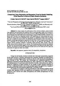
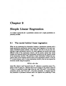
Ib'0-b 20 I ·' - 2 /e,+'/n +x -2 ~ ~st0, 86 1=0 tests C seem to excel, especially for larger values of 86 0 , This is of course the model for which test C seem to be not far behind, with B formance of test E' is also good, of the degrees of freedom must be

is designed. Tests Band E somewhat better than E. The perbut the possible overestimation borne in mind. Where 86 1>0, test B seems to give the best performance, especially for larger values of 86 1 , Table 3 gives the number of times each test gave a significant outcome when testing Ho (3) and Ho (4). For 86 0 >0, 861=0, test C gives the best performance by far, while A and D are next in line. In the case 86 0 =0, 86 1 >0 the test C shows a somewhat unexpected behaviour: In those cases where the tests could not show a difference between the slopes, it showed a difference between the abscissae (which did not exist) very easily. In this case test A seemed to be best. This is repeated in the case 86 0 >0, 86 1>0, where test C is, strictly speaking, not applicable. It is also seen that test D' (m unknown) is even somewhat better than D (m known) while it is nearly as good as test A. Thus it would seem best to use test D' when m is not known exactly and when the purpose is to find out whether the abscissae and/or the slopes are different. 7. Conclusion. From the Monte Carlo Study described in §6, it seems that the best test to use depends on the purpose and previous knowledge of the investigator: (a) if m=l, and the true lines are parallel the analysis of covariance test. seems best. (b) if m is known but the lines are not known to be parallel, the rejection region technique with joint estimates of 0 2 seems best. (c) if IT! is known only approximately, the rejection region technique with APDF seems preferable. The test with m unknown needs some attention because the true significance level seems higher than the nominal level.



47

_ . _ . TESTA

• • •

B E

0

0·2

_- - ...... ...........

..... ~ ••••••

0·' I.IJ ::l

a: ....

......

III

,--- ......

......

-16

-.

" , , ' _ ' -.&I • ..... :.~.: ••••••• :~.':"

/"-,,.,

0

I

l

2

3

4

z I.IJ

Fm

X ~

0 0·2 IIJ

....

0

IIJ ...., IIJ a: 0

0·'

X

tf1 ~

~

",-, I I ;(' ..,

m-O·36

" , ...................... . ...

'/:' .... ........ . ~--At;,...:::::::::::~~==========~~

,. "/

0"

o

~

'"~ ~

=",

" ......

- --

~

L __ _

~

0·6

_ _L __ _ _ _ _ _

~

2

______

.......

.........,;:

~

3

. .:::.-:-~ ~-....

______

~

____

~

44!5

GUESSED VALUE OF y and methodology in science and engineer>ing. John Hiley, New York. CHOH, G.C. (1960). Tests of equality between sets of coefficients in two linear regressions. Econometr>ica~, 591-604. ERLANDER, S. and GUSTAVSSON, J. (1965). Simultaneous confidence regions in normal regression analysis with an application to road accidents. Rev. Int. Statist. Inst. ~, 364-377. FINNEY, D.J. and SAMPFORD, M.R. (1961). The comparison of linear regressions for sets of correlated variates. Aust. J. Statist. ~,

1-19.

fRIEDt1AN, 14. (1937). Testing the significance among a group of regression equations. Econometr>ica~, 194-5. JANSSON, B. (1966). Random number> gener>ator>s. Victor Pettersons Bokindustri Aktiebolog, Stockholm. KASTENBAUM, M. (1959). A confidence interval on the abscissa of the point of intersection of two fitted linear regressions. Biometr>ics ~, 323-4. MILLER, R.G. (1966). Simultaneous statistical infer>ence. 14cGrawHill Book Co., New York.


CO~ARING

TWO REGRESSION LINES

53

TOCHER. K. (1952). On the concurrence of a set of regression lines. Biometrika ~, 109-117. WALKER, H.M. and LEV, J. (1953). Statistical inference. Henry Holt and Co., New York. WELCH, B.L. (1947). The generalization of Student's problem when several populations are involved. Biometrika~, 28-35. WILLIAMS, E.J. (1959). Regression analysis. John Wiley, Nevi York.

Manuscript received 22nd November 1967.


OPSOMMING VAN LESINGS

SUMMARY OF PAPERS

aangebied met die

presented at the

10 e Jaarlikse Kongres

lOth Annual

Congress

van die

of the

SUID-AFRlKAANSE STATISTIESE VERENIGING

SOUTH AFRICAN STATISTICAL ASSOCIATION

gehou

te

held at Scientiae

W.N.N.R. 26-27

C.S.I.R. Pretoria Oktober/October

1967

Statistics in South Africa J.E. Kerrich, Univepsity of the Witwatepspand. The author gives his personal opinion on (i)

the growth of statistics during the past 40 years, from very meagre beginnings;

(ii)

the present state of statistics in S. Africa. In particular, where are mathematical statisticians trained, what are they taught, how many are being trained and how are they employed;

(iii)

the growth of statistics in S.A. in the near future.

Apparently every university in S.A. now offers courses in Mathematical Statistics, although it is a comparatively new topic in most universities. Three universities reported that a total of 75 postgraduate degrees had been awarded in Statistics during the past five years. Six universities reported that among some 300 students who completed their third year undergraduate course in Mathematical Statistics, during the past three years, over 100 are continuing to study the subject, or have employment where they use statistics, or both. Strong doubt was expressed as to whether all employees use their statisticians to full advantage. It was felt that those who organise the teaching and use of Mathematical Statistics meet with very similar problems allover the world. Distribution-free confidence intervals for a shift parameter N.F. Laubscher, C.S.I.R., Pretopia. Let X1 , ••• ,Xm,and Y1 ' ••• 'Y n be two independent sets of rv's, the XIS iid with law FX(.) and the Y's iid such that X and y-9 have 55


OPSOMMINGS

56

identical distributions. A confidence interval for 6 is constructed which is based on the Wilcoxon rank sum statistic for testing difference in location between X and Y. The confidence interval is distribution-free in the sense that the confidence coefficient is independent of f X(')' An algorithm, based on the Mann-Whitney statistic, which is suitable for calculation on an electronic computer is provided. The method described has been briefly mentioned in the literature before but it is believed that it may now, with the aid of the computer, become a working proposition to be considered for use by research workers in applied fields. A worked example is included for comparative purposes with estimation also based on an obvious parametric technique. A theoretical study is envisaged to compare the efficiency of the above procedure with respect to standard parametric procedures (or competitive distribution-free methods) especially with regards to sequential usage (versus fixed sample size), cf. Robbins, Simons and Starr, Ann. Math. Stat. 38 (1967), 138~-1391. Toetsing van Normaliteit J.H. Venter, Potchefstroomse Universiteit vir C.H.O. Beskou In onafhanklike steekproef van grootte n uit In populasie met distribusiefunksie f. As toets vir die hipotese H : f(x) = o 9(x- U) vir een of ander ~ en cr, word die volgende voorgestel: cr = O·' stel Tn = Laat a1n, ••• ,a nn getalle wees so dat ~. a.I n n- 1 ~ a. i ln

x.ln

en S2 n

= i~(X.ln-xn )2

1

waar X1n , ••• ,X nn die rangorde

statistieke van die steekproef is en

Xn

die gemiddelde; stel ook

= n- 1 ~ a.ln EZ in waar Zln"",Znn die rangorde statistieke van Yn i

In onafhanklike steekproef van grootte n uit In N(O,l) verdeling is. Dan word H verwerp as T /S - y te veel van nul verskil. o n n n Die asimptotiese v~rdeling van die toetsgrootheid vir sommige keuses van die a. IS word bespreek met spesiale verwysing na die 1

l~

keuse a. = 9- (~). In n+l Dit word aan~edui dat die mag van die toets gunstig vergelyk met die van In X -toets. In Aantal onopgeloste probleme word gestel.

A statistical model to predict the efficiency of a colour sorter f.E. Steffens, C.S.I.R., Pretoria. In order to try and predict the performance of a colour sorter


57

SUMMARIES which might be used to remove impurities from a mineral during production. a few statistical models were investigated: at most one particle out of every n particles can be removed; after each particle removed, n-l particles have to pass the photo cell before the next impure particle is removed; and a modification of the latter model, stating that two particles are removed at a time. These models were investigated theoretically, and a simulation study was performed on each model.

Generalized inverse matrices and their statistical applications R.M. Pringle, University of Natal. Four types of generalized inverses can be defined for a matrix A. If Ag1 represents the set of all gl-inverses of A, AgZ the set of all g2-inverses, Ag 3 the set of all g3-inverses, and Ag the set of all the g-inverses,.then each of the four types is defined as follows:

=A

Ag'l

AAglA

Agz

AAgZA, AgzAAgz = Ag 2 I

Ag 3AAg 3 = Ag 3 (AAg 3) I = AAg3 AAgA = A, AgAA g = Ag , (AAg)I = AAg , (AgA) , = AgA AAg3A

= A,

Certain properties of these four types of generalized inverses, which have been described in the literature, are reviewed and the relationships betwee~ the four types have been discussed. In particular, it was shown t~at B is a g2-inverse of A if and only if B

=

P2

[~

where P1 and P 2 are non-singular matrices

[I,~

such that P1AP 2 = ~. ,'J ' r = r(A), and U and V are arbitrary. Alternatively, B is a g2-inverse of A if and only if B = G,AG 2 , where G1 , G2 e: Ag 1, As regards the statistical applications of g-inverses; for a normal vector Xl p~rtitioned as [ Xl x 2 ] " where x 2 haS singular variance matrix V22 ' the conditional mean and variance of Xl for fixed x 2 was expressed in terms of a g-inverse of V22 . Invariance under choice of g-inverse was shown. Finally, a further proof of the Gauss-Markoff theorem has been presented.

Oorsi

oor verdelin svr e variansie-analisemetodes C.F. Crouse, Universiteit van Sui -Afrika.

Die vernaamste probleem in die ontwikkeling van verdelingsvrye variansie-analisemetodes is om te toets vir interaksie-effekte onafhanklik van die hoofeffekte, In hierdie lesing is aangetoon hoedat hierdie probleem oorbrug kan ~ord in die geval van 'n 2n eksperiment en In 2 x k eksperiment met gelyke waarne-


OPSOMMINGS

58

mings in elke sel. Enige toets vir lokaliteit vir die geval van twee steekproewe kan na hierdie geval veralgemeen word. In besonder is aangetoon dat vir die Wilcoxon-tipe grootheid gee hierdie metode In asimptotiese relatiewe doeltreffendheid van 3/n relatief tot die t-toets in die geval van normaliteit.

An experiment in E.S.P. J. E. Kerrich, University of the flitwatersrand. A had 20 cards, alike in groups of 5, and drew them randomly one at a time. B, who knew this, guessed the type of card drawn. In 80 experiments mean no. of successes 7.32, with standard deviation sCm) = 0.27.

m=

Three standard methods of guessing not involving E.S.P. (Feller: "An Introduction to Probability Theory, Vol. 1, 2nd Ed., p. 99) were tested and rejected. Of-interest to statisticians is that it was quicker to simulate the probabilities associated with the thiTd method on an IBM 360 than to compute them from theory given in Joseph and Bizley "The two pack matching problem" J.R.S.S. Series B., Vol. 22, No.1, 1960. The non-central distribution of the largest root of the generalized B statistic D. J. de vlaal, University of the O. F. S. In this paper the non-central distribution of the largest root of the generalized a statistic in multivariate analysis is derived. To derive the distribution, it was necessary to evaluate a certain integral. This was done by using the Laplace transform and the convolution theorem. The central distribution of the largest root, as derived by Pillai (1967) (Ann. Math. Stat., 38, 616-617), follows as a special case of the non-central distribution by taking the non-centrality parameter equal to zero. The non-central distribution of the smallest root is also derived which follows easily from the distribution of the largest root by using a simple substitution. Studies in wiskundige sosiologie H.S. Steyn en G. Gerntholtz, Universiteit van Suid-Afrika. Sedert 1966 is personeellede van die Departemente Wiskundige Statistiek en Sosiologie aan die Universiteit van Suid-Afrika besig om in same werking met die Nasionale Buro vir Opvoedkundige en Maatskaplike Havorsing die bestaande literatuur oor Wiskundige Sosiologie stelselmatig na te gaan. Enkele navorsingsprojekte van teoretiese sowel as van praktiese aard word onderneem. Daar bestaan In verskeidenheid van modelle deur skrywers soos Simon, Katz, Harary, Cartwright en andere. Differensiaalvergelykinge, grafiekteorie en matriksalgebra speel, onder andere, In groot rol in die opstelling van die modelle. Sekere uitbreidings deur die skrywers van Katz se modelle vir die berekening


SUMMARIES van statusindekse het reeds vrugbare resultate gelewer. Lineere programmeringstegnieke en faktorontledingstegnieke hou goeie belofte in vir vrugbare toekomstige gebruik in die Wiskundige Sosiologie. Voorbeelde van die toepassing van statusmodelle en die berekening van statusindekse word behandel. Oorgangsbenaderings tot die steekproefverdeling van die gemiddelde uit Pearson-tipe-populasies G.P. Viljoen, Universiteit van die o. v.s. Alhoewel die normaalverdeling na aanleiding van die sentrale limietstelling gewoonlik gebruik word as In benadering vir die steekproefverdeling van die gemiddelde vir steekproewe uit enige populasie, het Berry in 1941 aangetoon dat dit ontoereikend is. In In poging om die gaping tussen die eksakte verdeling van die gemiddelde en sy uiteindelike normale benadering te oorbrug, het In aantal ondersoekers benaderings tot hierdie verdeling voorgestel. O.a. het Esseen in 1945 die tipe A reeksverdeling voorgestel, terwyl Welker in 1947 benaderings tot die Pearsonstelsel en Daniels in 1954 die sogenaamde saalpunt-benaderings afgelei het. Hierdie benaderings is egter nie bevredigend nie. In hierdie studie \-lord gepoog om die gaping te oorbrug d.m.v. verdelings \-Iat as benaderings gebruik kan word en wat ook in mekaar oorgaan. Die Besselfunksie-verdeling gaan bv. oor in die gammaverdeling, wat op sy beurt weer oorgaan in die normaalverdeling. Toepassing van Van Dantzig se metode van kollektiewe kenmerke in verdelingsvryemetodes D.J. Stoker, Universiteit van Pretoria. Die kollektiewe kenmerk van In waarskynlikheidsverdeling kan beskou \-lord as In veralgemening van waarskynlikheid- en momentvoortbringende funksies. Deur gebruikmaking van die met ode van kollektiewe kenmerke, wat deur D. van Dantzig ontwikkel is, kan belangrike resultate dikwels op In kort en elegante wyse verkry word. Die toepassing van genoemde metode is op In drietal probleme uit die verdelingsvryeteorie geillustreer, nl. om uitdrukkings te verkry vir die verwagtingswaarde en variansie van In algemene funksie van die rangnommer toegeken aan In waarneming in In bepaalde sel van In blokontwerp (wat volledig of onvolledig, gebalanseerd of niegebalanseerd kan wees) onder In klas van a.r.d.-tipe alternatiewe hipoteses; en om die karakteristiekefunksie, onder die nulhipotese, van die rangkorrelasiekoeffisient van Kendall en van die Utoetsgrootheid van Mann-Whitney-Wilcoxon in die tweesteekproefprobleem te verkry.