Simple PID Tuning Rules for Varying Time-Delay Systems

Publication [P7]

L. M. Eriksson, M. Johansson, “Simple PID Tuning Rules for Varying TimeDelay Systems”, in Proc. The 46th IEEE Conference on Decision and Control (CDC 2007), New Orleans, LA, USA, December 12-14, 2007, 7 p. © 2007 IEEE. Reprinted, with permission.

This material is posted here with permission of the IEEE. Such permission of the IEEE does not in any way imply IEEE endorsement of any of Helsinki University of Technology's products or services. Internal or personal use of this material is permitted. However, permission to reprint/republish this material for advertising or promotional purposes or for creating new collective works for resale or redistribution must be obtained from the IEEE by writing to [email protected]. By choosing to view this document, you agree to all provisions of the copyright laws protecting it.

Simple PID Tuning Rules for Varying Time-Delay Systems Lasse M. Eriksson and Mikael Johansson

Abstract— This paper discusses tuning of PID controllers for varying time-delay systems. We analyze the properties of the AMIGO tuning rules of Åström and Hägglund applied to varying time-delay systems and propose improved tuning rules which increase the robustness to delay variations at the expense of a small degradation in nominal performance. We suggest a tuning scheme that uses the simple AMIGO tuning on an extended plant, and define the design concepts for extending the plant. This approach allows treating the maximum time-delay as a design parameter for the tuning rules. The proposed tuning rules are compared via simulations.

A

I. INTRODUCTION

NY practical control system suffers from delays. These can stem from process dynamics, actuators or sampling. The delays are often either assumed negligible or constant, but in some cases the variance in delay times (jitter) plays a significant role. There exists a variety of methods for control of time-delay systems with constant delays, but the toolset for dealing with varying time-delays is much more limited. While time-delay systems are abundant in practice, our work is partly motivated by the emerging technology of networked control. There is strong current desire to develop technologies that allow a transition from today’s wired infrastructures to more flexible and cost-efficient wireless automation systems. This “wireless migration” requires significant advances in a wide range of technologies, including wireless communication, networking, software engineering, and control. Our focus is on the design of practical controllers that are robust to the varying time-delays incurred by unreliable communications. The PID (proportional-integral-derivative) controller is the most common controller in industrial applications today, and it is likely to be the most important controller also in wireless automation solutions. There are many different architectural options for networked PID controllers, including the use of “network observers” [1] to compensate for delay, jitter, losses and other network deficiencies, or simply keeping the architecture of the wired controller and modifying the controller parameters. This paper takes the second path, and develops new tuning rules that aim at providing good time-domain performance while being robust to varying time-delays. Recently, the PID tuning problem for varying time-delay

systems has been approached using multi-objective optimization to develop rules that maximize the jitter margin, i.e. the maximum value of any additional varying time-delay in the control system [2], [3]. This approach might result in complicated rule structures, which only apply for a certain range of process parameter values. In this paper, we extend the simple AMIGO (Approximate M-constrained Integral Gain Optimization) tuning rules [4], [5] that have been developed for PID tuning in process control, such that varying time-delays are better taken into account while adhering to the simple rule structures. There are AMIGO rules for nonintegrating and integrating processes, but we only consider non-integrating processes. The integrating processes are treated in [3]. We consider extending the plant with a well designed measurement filter before applying the AMIGO design on the extended plant. This approach allows using the required jitter margin as a parameter to the tuning rules. In the next section the basic concepts and preliminaries required to understand the problem and the proposed tuning approach are presented. The AMIGO tuning that is frequently referred to in the paper is also presented in Section II. Based on the AMIGO tuning analysis presented in Section III, we propose an extended plant design approach and filter design concepts that better fit for varying time-delay systems in Section IV. Section V compares the proposed tuning and Section VI analyses the delay-dominant processes separately. Simulation results are presented in Section VII and Section VIII states the conclusions. II. PRELIMINARIES A. PID Controller The PID controller is the most common controller used in industry. There are several versions of the basic algorithm t ⎛ 1 de(t ) ⎞ u (t ) = K ⎜ e(t ) + ∫ e(τ )dτ + Td ⎟, (1) Ti 0 dt ⎠ ⎝ e(t ) = yr (t ) − y (t ),

where u is the control signal, e the error signal, yr the reference signal, y the process variable, K the gain, Ti the integration time, and Td the derivative time. In this paper we consider the following version of the PID controller, since the “text book” version (1) is very sensitive to noise. t

L. M. Eriksson is a Ph.D. student with the Control Engineering Laboratory, Helsinki University of Technology, P.O.B. 5500, Espoo, FI-02015 Finland (e-mail: [email protected]). M. Johansson is an associate professor with the Automatic Control, Royal Institute of Technology, Stockholm, SE-10044 Sweden (e-mail: [email protected]).

u (t ) = k ( byr (t ) − y f (t ) ) + ki ∫ ( yr (τ ) − y f (τ ) )dτ 0

⎛ dy (t ) dy f (t ) ⎞ + kd ⎜ c r − ⎟ dt dt ⎠ ⎝

(2)

Here k, ki, and kd are the controller gains, b and c the setpoint weights, and yf is the filtered process variable such that 1 Y f ( s ) = G f ( s )Y ( s ) = Y ( s) , (3) (1 + sT f ) n where Y(s) is the Laplace transform of the process variable y(t). Tf is the measurement filter time-constant and n the order of the filter. Typically n equals one or two. B. Jitter margin There exists a variety of stability results for varying timedelay systems (see e.g. [6]). Most of the theorems are in time domain, but there are also certain frequency domain criteria such as [7]. The criteria presented in [7] are based on the assumption that the varying time-delay is bounded. The upper bound for the delay is called the jitter margin. The delay can be of any type (constant, time-dependent, random), but the jitter margin determines the upper bound for it. The formal definition of the jitter margin is given in [7], where three different controller/plant–uncertainty combinations in continuous- and discrete-time are investigated. The first one is shown in Fig. 1, left, where a continuous-time plant and a continuous-time controller with controller output uncertainty are shown. This continuous-time SISO system is stable for any time-varying delays defined by Δ (v) = v ( t − δ (t ) ) , 0 ≤ δ (t ) ≤ δ max (4) if P ( jω )C ( jω ) 1 < , ∀ω ∈ [ 0, ∞[ , 1 + P ( jω )C ( jω ) δ maxω

(5)

where δmax is the jitter margin. The proof of the result is based on presenting the uncertainty (varying time-delay) with an operator Δ F := ( Δ − 1) D 1 s (s being the Laplace operator) and on the small gain theorem. However, in this paper the jitter is assumed to be after the plant (e.g. sampling jitter) as depicted in Fig. 1, right. Since the signals in the control loop are all continuous, and only the plant and controller switch their positions, the small gain theorem-based stability proof, and the resulting criterion (5), still hold for the control system in Fig. 1, right. C. AMIGO tuning rules The objective of this work is to develop simple tuning rules for the PID controller in varying time-delay systems. The AMIGO tuning rules [4], [5] were selected as the point of comparison, since they provide good performance and are robust to disturbances in control systems without varying time-delays. The AMIGO tuning rules are based on approximating the process with the so-called KLT-process model (first order lag plus delay) possibly determined via a simple step experiment, see [4]. The tuning rules are obtained from the KLT-parameters. The most well-known step response based tuning rules were presented by Ziegler and Nichols already in 1942 [8]. The KLT-process model is K p − sL PKLT ( s ) = e , (6) 1 + sT

yr

+ _

P(s)

Δ

yr

+ _

C(s)

Δ C(s)

P(s)

Fig. 1. Continuous-time controller (C) and plant (P) with an uncertain timevarying delay (Δ) in the feedback loop. On the left, Δ is the controller output uncertainty. On the right, Δ is the process output uncertainty.

where Kp is the static gain, T the time-constant, and L the (constant) time-delay. The AMIGO rules were developed by analyzing different properties (performance, robustness etc.) of a process test batch with over 130 processes, and the resulting tuning rules are 1 ⎛ T⎞ K= ⎜ 0.2 + 0.45 ⎟ , Kp ⎝ L⎠ 0.4 L + 0.8T L, (7) L + 0.1T 0.5LT Td = . 0.3L + T In order to use the PID controller with filtering (2), the rules are extended as follows [4]: ⎧ ⎧0, if τ ≤ 0.5 ⎧k = K ⎪b = ⎨ ⎩1, if τ > 0.5 ⎪ ⎪ K ⎪ ⎪ (8) ⎨ ki = ⎨c = 0 Ti ⎪ ⎪ ⎪ ⎪T = ⎧⎨0.05 / ω gc , if τ ≤ 0.2 ⎩kd = K ⋅ Td ⎪⎩ f ⎩ 0.1 ⋅ L, if τ > 0.2. Here τ refers to the relative dead time of the process L τ= , (9) L +T which has turned out to be a significant process parameter when controller tuning is considered, and ωgc is the gain crossover frequency. The development of the AMIGO rules was based on the following robustness criterion: if the Nyquist curve of the loop transfer function does not intersect a circle with center cR and radius rR defined as 2M 2 − 2M + 1 2M − 1 cR = − , rR = , (10) 2 M ( M − 1) 2 M ( M − 1) Ti =

then the sensitivity function and the complementary sensitivity function are less than M [9]. The robustness is thus captured by one parameter only, M. The value M = 1.4 was used in the AMIGO rule development, although finally the rules did not quite satisfy the constraint. For the process test batch a 15 % increase of M was reported (M ≈ 1.6). III. ANALYSIS OF THE AMIGO TUNING In [2] the jitter margin properties of AMIGO tuning are examined. It is shown that the jitter margin of a pure KLTprocess with AMIGO tuned controller (2) is approximately δmax, AMIGO ≈ 0.71⋅L. It is also suggested in [2] that the measurement filter time-constant Tf might have a great impact on

where L ( 0.4 L + 0.8T )( 0.3L + T ) , γ= 0.2 + 0.45 T L (12)

κ = L ( 0.3L + T )( 0.4 L + 0.8T ) , λ = ( L + 0.1T )( 0.3L + T ) .

It seems that (11) does not have an analytical solution, which could possibly give more insight on the dependency of jitter margin on the process parameters. Numerically, though, the expression is trivial to solve if a sufficiently wide frequency range is used. Some remarks can be made on (11). If the measurement filtering is not used, i.e. Tf = n = 0, we get 1 + jωT

e

− jω L

(ηω

2

+ jκω + λ )

KLT+PID w/o filter 10 5

+

1 → 0. jω ω →∞

(13)

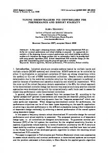
This means that the jitter margin is zero for a KLTprocess with PID controller without measurement filtering. The reason for this is the fact that the system does not have roll-off at high frequencies. This can be verified from the closed-loop system’s Bode diagram, which corresponds to the left side of inequality (5). In Fig. 2, a KLT-process with parameters Kp = 1, T = 3 and L = 1 in conjunction with an AMIGO-tuned PID controller with and without the measurement filter are considered. The solid line represents the system’s frequency response amplitude in the case without the filter. The dotted line intersecting the solid line represents the jitter margin criterion (right side of (5)) with δmax = 0.5. Obviously, the jitter margin criterion is not satisfied in this case. For comparison, the dash-dotted line shows the frequency response amplitude for the system with the measurement filter that is tuned according to the AMIGO rules. For the system with the filter, the jitter margin requirement is clearly satisfied. The above analysis verifies the need for the measurement filter in varying time-delay systems. In addition, the filter naturally reduces the effect of measurement noise and it is often considered a prerequisite for using the derivative part of the PID controller in practical control systems. Still it remains unclear if the AMIGO tuning rule for Tf is optimal in jitter-sense.

1/(δmax ω) KLT+PID w. filter

0 -5 -10 -15 -20 -25 -30 -4 10

η = −0.5L2T ( 0.4 L + 0.8T ) ,

δ max < γ

Closed-loop Bode-plots and 1/(δmax ω) for δmax = 0.5 15

Magnitude (dB)

the jitter margin. To further explore the jitter margin properties in this case the analytical jitter margin formula is derived here. Consider the pure KLT-process (6) and the controller (2), where the parameters k, ki and kd are tuned according to AMIGO tuning rules (7) and (8). The jitter margin δmax solved from (5) becomes 1 + P ( jω )C ( jω ) δ max < jω P ( jω )C ( jω ) (11) n (1 + jωT ) (1 + jωT f ) 1 = γ − jω L + , ∀ω ∈ [ 0, ∞[ ⎡⎣ηω 2 + jκω + λ ⎤⎦ jω e

-3

10

-2

10

-1

10 Frequency rad/s

0

10

1

10

2

10

Fig. 2. Closed-loop Bode diagram of a KLT+PID system with and without the measurement filter.

The discussion above motivates a more thorough evaluation of how the measurement filter time-constant affects the jitter margin of AMIGO rules. Obviously, the value of Tf should not be dominant in the control system, i.e. it should be relatively small compared to the process dynamics (timeconstant and delay). If the filter time-constant was dominant in the system, losses in performance would be expected. To better analyze the relationship between Tf and δmax, the jitter margins for a range of KLT-processes with AMIGO-tuned PID controller and different filter time-constants Tf are calculated. Kp can be omitted from the analysis, since it is cancelled by the controller. Fig. 3 shows the jitter margin for various values of the process parameters as a function of Tf. The batches of curves in Fig. 3 represent the jitter margin for certain value of delay (here L = 2, 6 and 10 are used for the example). Each curve in one batch corresponds to certain value of process time-constant, T. From the figure it is seen that the jitter margin is not greatly affected by the process time-constant for the relevant range of (small values of) Tf. Another remark is that the jitter margin seems to have a certain maximum value in the range where Tf is relatively small. A closer look at the curves reveals that the value of Tf maximizing the jitter margin is nearly independent of process time-constant T (see the circled positions in the figure). Further analysis shows that the optimal value of Tf is linearly dependent on L and that a very simple tuning rule for Tf could be derived. Using numerous values for L and T in the range [0.1 10] and parameter estimation, the optimal value of the measurement filter time-constant was identified as T f* ≈ 0.17 L . (14) Although this value of Tf differs only slightly from the AMIGO tuning rule (Tf = 0.1⋅L for τ > 0.2), it has a significant effect on the jitter margin. Whereas the jitter margin for AMIGO tuning is approximately 0.71⋅L, (14) gives jitter margins 1.16⋅L…1.25⋅L depending on the value of T. Thus, an increase of up to 75 % in jitter margin could be achieved by this simple modification for the pure KLT-process.

δmax with respect to Tf for KLT+AMIGO with T = [0.1...10] 14 L=2 L=6 L = 10

12 10

δmax

8 6 4 2 0 0

5

10

15 Tf

20

25

30

Fig. 3. The jitter margin of KLT-process with AMIGO tuning as a function of measurement filter time-constant Tf.

This tuning rule was tested with the same process test batch that was used in the derivation of AMIGO rules (see [4] and [5] for details). The batch consists of 133 processes of nine different types. The jitter margin and the ITAE performance criterion were compared to see how the change of filter tuning rule affects robustness and performance. For the pure KLT-processes and those that are “close” to KLT in the test batch, the tuning rule (14) gives excellent results, i.e. better jitter margin without sacrificing the performance. For other processes the jitter margin remains almost equal to the values provided by the AMIGO tuning. The performance of the control systems remains at approximately equal level to AMIGO. Since this very simple modification of the AMIGO tuning rules does not guarantee better jitter margin and performance for all processes, we next consider a complete measurement filter re-design to reach these objectives. IV. EXTENDED PLANT DESIGN APPROACH This section discusses a new way of designing and tuning the filter for the AMIGO tuning rules. The main idea in this approach is to allow the desired jitter margin to be an input to the tuning rules, which enables adjusting the controller performance according to the requirements posed by the control system. For instance, this would be very useful for networked control systems, where often good estimates of the maximum delay can be given. The question is how to tune the controller such that the criterion (5) is satisfied for the specified jitter margin. Simple tuning rules for which the maximum delay can be directly assigned would be desirable in many practical cases. In this section we propose such tuning schemes. In AMIGO tuning the process is approximated by the KLT-model. In the previous section we concluded that the maximum achievable jitter margin for a pure KLT-process with AMIGO tuning using (14) gives δmax ≈ 1.2⋅L with reasonably small values of the filter time-constant. Especially for lag dominated processes, for which T >> L, the requirement for the jitter margin might be considerably bigger than

the mentioned constraint. Thus the design approach needs to be revised. We propose a method where the measurement filter is first designed based on the required jitter margin, and then the plant is extended with the filter before approximating the KLT-model of the extended plant, Pext(s) = Gf(s)P(s). The PID controller parameters are calculated using the extended plant’s KLT-approximation and the standard AMIGO rules except for the filter time-constant (which is already in the system). Consider the KLT-process model with a PID controller. As shown before, the jitter margin is hard to solve analytically even for this simple process model case. Nevertheless, using well-justified approximations the analysis is significantly eased. At high frequencies the following approximations are valid. P( jω )C ( jω ) ≈ P ( jω )C ( jω ) 1 + P ( jω )C ( jω ) =

Kp 1 + jωT

e

− jω L

K p kd ⎛ ⎞ ki + kd jω ⎟ → . ⎜k + jω ⎝ ⎠ ω →∞ T

Using the AMIGO tuning rule for kd in (15) results in K p kd 0.1L + 0.225T 1 = ≈ . 0.3L + T 3 T

(15)

(16)

As seen in Fig. 2 and in (16), at high frequencies the frequency response amplitude of the KLT-model with PID controller without the filter remains approximately constant. If the system has the filter, it dominates the system behavior at high frequencies. In order to make the analysis general, we let the measurement filter order n vary and consider cases n = 1 and n > 1 separately. Based on (16) the jitter margin of the system with an nth order measurement filter becomes

δ max

(1 + jωT ) 1/3δmax. Since small values of Tf are preferred, we finally set the tuning rule as 1 T f = δ max . (19) 3 Similarly, for n > 1 we have

δ max
3 n ⎜ ⎟ ⎝ n −1 ⎠

( n −1)

2

Growth percentage of the jitter margin compared to AMIGO

Tf .

300

(22)

V. COMPARISON OF THE NEW RULES This section compares the tuning rules presented above. We restrict to cases where n = 1, 2, 3 to avoid unnecessary highorder controllers. The rules use the extended plant approach where the required jitter margin can be given as an input parameter for the design. The proposed design approaches are compared with respect to AMIGO tuning in Fig. 4 and Fig. 5. We use the AMIGO process test batch and restrict to stable processes (integrating processes P6 are omitted). The ITAE criterion is used as the performance measure throughout the study. Fig. 4 shows the relative improvement in jitter margin compared to AMIGO tuning for the test batch. For the extended plant approaches the objective value for the jitter margin is twice as large as the jitter margin of the AMIGO tuned process, i.e. the dots in Fig. 4 should all be aligned at 100 %. Fig. 5 shows the relative ITAE cost criterion values of the new tuning rules with respect to those of AMIGO tuning. Here the value 0 % corresponds to the performance achieved with AMIGO tuning, and positive values indicate performance losses when applying the new rules. For most of the processes the extended plant approaches give promising results, and the improvements in jitter margins are close to 100 %. Problems arise for processes with T < L, i.e. delay-dominant processes. These processes are further studied in Section VI. As far as the jitter margin is considered, the third-order filter appears to give the most accurate results for the test batch, although the ITAE criterion increases the most for the third-order filter. In general, the ITAE increases the most for slow processes with large T. The increase of ITAE seems in some cases quite significant, but this might also stem from the time-weighting in the criterion: if the performance of a process with large T is decreased in order to achieve bigger jitter margin, the settling time of the process increases. The longer the settling time, the more ITAE criterion punishes for error. Since the time is integrated, its effect is not linear, but rather squared.

200 150 100 50 0

P1

P2

P3 P4 P5 P 6

P7

P8 P 9

-50 -100

0

20

40

60 80 Process number

100

120

140

Fig. 4. The jitter margin growth percentage compared to AMIGO tuning in the test batch. ITAE criterion compared to AMIGO in percentages 200

ITAE cost criterion w.r.t AMIGO in %

(1− n ) 2

1 ⎛ n ⎞ δ max . (23) ⎜ ⎟ 3 n ⎝ n −1 ⎠ Hence we have the design rules for the measurement filter with n ≥ 1. To arrive at a complete PID-tuning, we propose to first design the measurement filter (of desired order) using the rules above, and then include the filter dynamics in the plant and apply the AMIGO tuning on the extended plant to calculate the remaining controller parameters (k, ki, kd, b and c). The previously designed measurement filter is then used in the controller. The filter order may be restricted by the process or measurement noise properties. If a high-order filter is used, losses in performance are presumable. In the next section, the proposed filter design guidelines are compared in performance and in jitter margin.

Growth of δmax w.r.t AMIGO in %

Solving (22) for Tf leads to the tuning rule Tf =

n=1 n=2 n=3

250

n=1 n=2 n=3

150

100

50

0

-50

P1

0

P2

20

P3 P4 P5 P 6

40

60 80 Process number

P7

100

P8 P 9

120

140

Fig. 5. The relative ITAE cost criterion with respect to the AMIGO tuning in the test batch.

VI. DELAY-DOMINANT PROCESSES The results in Fig. 4 indicate that the extended plant approach might have some fundamental limitations for delaydominant processes. The performance of the tuning rules is modest for processes for which T < L, where the variables refer to the plant’s KLT-approximation parameters. The above presented problems gave reasons for investigating the extended plant approach generally for delaydominant processes. The behavior of the jitter margin with respect to the filter time-constant was examined using the extended plant approach similarly as was done in Fig. 3 for the standard AMIGO tuning. This study was done with KLT-parameters in the ranges T = [0.02…1] and L = [1, 2]. Fig. 6 shows an example of the results with parameters T = 0.5 and L = 1 for n = 1, 2, 3, but consistent behavior was observed for all parameter combinations tested. As seen in Fig. 6, for n = 1, the jitter margin has an upper bound and increasing Tf does not increase the jitter margin infinitely. The upper bound is independent of L at least when T