Haw-Shiuan Chang and Yu-Chiang Frank Wang. Research ...... Belongie, S., Carson, C., Greenspan, H., Malik, J.: Color-and texture-based image segmen-.
Simple-to-Complex Discriminative Clustering for Hierarchical Image Segmentation Haw-Shiuan Chang and Yu-Chiang Frank Wang Research Center for Information Technology Innovation, Academia Sinica, Taipei, Taiwan
Abstract. We propose a novel discriminative clustering algorithm with a hierarchical framework for solving unsupervised image segmentation problems. Our discriminative clustering process can be viewed as an EM algorithm, which alternates between the learning of image visual appearance models and the updates of cluster labels (i.e., segmentation outputs) for each image segment. In particular, we advance a simple-to-complex strategy during the above process, which allows the learning of a series of classifiers with different generalization capabilities from the input image, so that consecutive image segments can be well separated. With the proposed hierarchical framework, improved image segmentation can be achieved even if the shapes of the segments are complex, or the boundaries between them are ambiguous. Our work is different from existing region or contour-based approaches, which typically focus on either separating local image regions or determining the associated contours. Our experiments verify that we outperform state-of-the-art approaches on unsupervised image segmentation.
1
Introduction
With the goal of partitioning an image into several spatially coherent regions, image segmentation has been a fundamental computer vision task, which benefits a variety of applications such as object recognition [1,2,3] and video object segmentation/tracking [4,5,6]. Generally, challenges of image segmentation lie in the diversity and ambiguity of visual patterns presented in images. Therefore, without any prior knowledge or user interaction, optimal image partition might not be easily determined in an unsupervised way. As suggested in [7,8], one can divide existing unsupervised segmentation algorithms into two categories: region [9,10,11,12,13] and contour-based [14,8,15,16] approaches. The former considers the input image as a graph, in which each node represents a pixel or an image segment, while the edges connecting each node pair indicate the associated similarity. Thus, the problem of image segmentation turns into a clustering task, which can be solved by techniques like normalized cut (NCut) [9]. To better deal with image segments at different scales, more advanced graph representations have been proposed for improved segmentation (e.g., MNCut [10], correlation clustering [11], SAS [12], FNCut [13]). Instead of merging local image regions into segments, contour-based approaches aim at exploring local image regions for determining the object boundaries [14,8,15,16]. This type of methods design classifiers for identifying image contours using feature
2
Haw-Shiuan Chang and Yu-Chiang Frank Wang
(a)
(b)
(c)
(d)
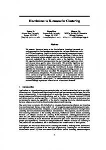
Fig. 1: Illustration of region and contour-based approaches. (a) Input image, (b) region-based output by SAS [12], (c) contour-based output by gPb [8], and (d) ours by advancing both region and contour information with a hierarchical segmentation framework.
cues like color or texture (e.g., gPb [8]), and thus image segments can be estimated accordingly (e.g., OWT-UCM [8] or Multicut [15]). However, contour-based approaches might not generalize well if there exist large scale changes for the objects presented in the input image [8]. In addition, contour detection might fail in determining object edges for blurry or articulated regions. Therefore, recent approaches like SWA [17,18], gPb-OWT-UCM [8], or ISCRA [16] advocate an agglomerative clustering (bottom-up) strategy for alleviating the above problems by performing segmentation from finer to coarser image scales. However, as pointed out in [16], if one cannot properly update the contour information during the above hierarchical process (e.g., contour probability of gPb-OWT-UCM only determined at the bottom level), the resulting segmentation performance would still be limited. As noted in [19,20], successful image segmentation would benefit from feature cues extracted beyond local regions. For local image regions with sufficient and distinct feature information, although promising results have been reported by state-ofthe-art methods like gPb-OWT-UCM, human segmentation still achieves much better performance due to the consideration of information extracted beyond local contours. As studied in [20], this is because that human tends to consider feature cues from nonlocal regions (e.g., those farther away from the detected contours) when performing segmentation, even he/she does not recognize the object presented in the input image. Motivated by the above observations, we propose a novel framework for unsupervised hierarchical image segmentation. Our approach utilizes contour detection at different image scales as initialization, and unsupervised image segmentation is achieved by an EM-like iterative algorithm, which essentially performs discriminative clustering and maximizes the separation between consecutive image regions. The proposed hierarchical segmentation process is able to integrate both local and global (non-local) statistics for improved segmentation. As depicted in Figure 1, improved segmentation can be expected by our proposed approach. In our discriminative clustering process, we advocate a simple-to-complex strategy for learning a series of classifiers with different generalization capabilities at each image scale. This unique technique allows us to adaptively separate consecutive object regions by maximizing the differences between the associated feature distributions.
Simple-to-Complex Discriminative Clustering for Hierarchical Image Segmentation Discriminative Clustering
l=L
Clusters
Ground Truth
Original Image
Segments at Level l+1
Hierarchical Segmentation
l=1
3
Segments at Level l
EM-like Optimization m m+1 ...
Segments s
...
s+1
Contour Detection
s+2
s+3
Initial Clusters
Fig. 2: Our proposed hierarchical image segmentation framework.
1.1
Our Contributions
– Starting from contour detection, our hierarchical segmentation framework advances graph-based clustering which exploits and integrates local and non-local feature cues for unsupervised segmentation. – The proposed simple-to-complex discriminative clustering strategy allows automatic learning of a series of classifiers, which exhibit different generalization capabilities for discriminating between image segments, while no additional training process or data are needed.
2 2.1
Our Proposed Method Hierarchical Image Segmentation
As illustrated in Figure 2, we advance a hierarchical (i.e., bottom-up) framework for unsupervised image segmentation, in which we consider the clustering outputs at each image scale as the input segments for its upper (coarser) level in the hierarchy. For the interest of computation efficiency, instead of performing pixel-level segmentation at the starting bottom level l = 1, we over-segment the input image and start the hierarchical process using superpixels. We apply Turbopixel [21] for performing over-segmentation, which is able to produce compact superpixels with similar sizes (we fix the number of superpixels N as 1200 in our work). Since we do not assume the number of clusters known at each level l, we fix the ratio of the numbers of clusters K in consecutive scales as r = 1/2, and this hierarchical segmentation process would terminate once the minimum number of clusters allowed is reached. Our proposed segmentation process is summarized in Algorithm 1. In the following subsections, we will detail how we observe multiple feature cues for performing unsupervised segmentation in each level of our hierarchical framework. 2.2
Discriminative Clustering via EM Optimization
As noted above, we view the segmentation output of a lower level in the hierarchy as the input of the current level. We now discuss how the segmentation at each level can be viewed as solving a graph-based optimization task.
4
Haw-Shiuan Chang and Yu-Chiang Frank Wang
Algorithm 1: Our Proposed Segmentation Framework Input: Image I, ratio r, maximum iteration number kmax l Output: Segments sl and contour probability Pcontour for each level l in the hierarchy Over-segmentation step: Over-segment I and produce superpixels sl1,...,K , where level l ← 1, K ← Number of superpixels N while K > 1 do Discriminative clustering step: l Pcontour ← Detect contours between sl1,...,K l+1 s1,...,dK×re ← Initially cluster sl1,...,K by NCut for Iteration k = 1 to kmax do M-step: Construct probability models for each cluster m Pck (i|m) (1), Ptk (i|m) (3), P k (ps |m) (5) E-step: ml1,...,K ← Classify sl1,...,K by minimizing E l in (8) l l sl+1 1,...,dK×re ← Merge s1,...,K by m1,...,K Simple-to-complex step: Updating σ (1), wt,k (4), wk (7) for classifier models in each feature space K ← dK × re and l ← l + 1
Take level l in the hierarchy for example, we start from determining the probability l for the edges between image segments being object contours, as depicted PContour in Figure 2. These probabilities are calculated by the differences of texture and color distributions between consecutive image segments using χ2 and Earth Mover Distances (EMD) [22,23], respectively. Different from mPb [14,8], we do not consider the use of any training data for estimating such probabilities. With image segments and the associated contour probabilities are obtained, we apply NCut [9] for performing graphbased optimization. This would separate the input segments from K into K ×r clusters, which will be viewed as initial segmentation results as shown in Figures 2 and 3. Since graph-based segmentation techniques like NCut are known to produce clusters (i.e., image segments) with similar sizes [12], complex or ambiguous image regions might not be properly separated. This is why we advance discriminative clustering in our proposed framework, aiming at the refinement of the clustering/labeling outputs at each level in our hierarchy. For the task of unsupervised segmentation, separation between clusters needs to be automatically achieved by observing the features/classifiers from consecutive image segments. For discriminative clustering in our proposed segmentation method, we propose to learn of a series of classifiers with different generalization capabilities for refined image segmentation. More precisely, each image cluster (i.e., a set of image segments with the same label) will be recognized by a particular classifier, which will be automatically learned from the input image data using multiple types of features. Essentially, our discriminative clustering strategy can be considered as an EM-like process, which is summarized as follows:
Simple-to-Complex Discriminative Clustering for Hierarchical Image Segmentation
5
Simple to Complex
Color
Iteration k=kmax
Iteration k=1 Color
Texture
...
...
Locality Original Image
Clusters m=1 Clusters m
s
Segments at Level l
m+1
s+1 s+2 s+3 ...
Segments Initial Clusters
...
...
˥K×r ˥
Texture
Clusters m=1
...
Clusters m
m+1
...
}
M-step
...
Locality
˥K×r˥
...
}
E -step
s
s+1 s+2 s+3 ...
Segments
Segments at Level l+1
Fig. 3: Our discriminative clustering process with a simple-to-complex strategy at level l in the hierarchy (K is the number of segments).
– M-step: Given the clustering outputs, construct the probability model of each image cluster in different feature spaces – E-step: Given the observed cluster models, classify each image segment into the corresponding cluster based on the estimated probabilities Although prior works on foreground object segmentation like GrabCut also utilized similar iterative clustering techniques [24,4,5,6,25], they typically required additional efforts or information for annotating foreground/background regions (e.g., user interaction or use of temporal features), otherwise the associated classifiers cannot be easily derived. On the other hand, while EM-based image segmentation has been previously explored in [26,27,28], such methods still require proper selection of parameters (e.g., the number of segments) for performing segmentation. In our work, we focus on unsupervised image segmentation. At each scale in the hierarchy, our proposed segmentation algorithm is able to discriminate between consecutive segments using classifiers with different generalization capabilities. These classifier models will first be observed at the M-step of each iteration, and they will be applied to separate image segments at the following E-step. In Section 2.3, we will detail how we apply a simple-to-complex strategy for discriminative clustering in our hierarchical segmentation framework. 2.3
Simple-to-Complex Classification and Segmentation
As depicted in Figure 3, our simple-to-complex strategy for discriminative clustering first observes simpler classifiers (e.g., kernel density estimation based classifier with larger σ) at the M-step of each iteration. This results in coarser separation between image segments at the E-step by updating the cluster labels. With this simple-to-complex strategy, it will be less likely for segmentation outputs to overfit the initial contour detection results in the beginning of the segmentation process. For the subsequent iterations, we treat the newly-predicted segment pairs as updated training data, and we re-design the classifiers with increased complexities (e.g., smaller σ for Gaussian kernels). Figure 4 illustrates our proposed simple-to-complex strategy. It is clear that, our
6
Haw-Shiuan Chang and Yu-Chiang Frank Wang 1
1
1
1
1
0.8
0.8
0.8
0.8
0.8
0.6
0.6
0.6
0.6
0.6
0.4
0.4
0.4
0.4
0.4
0.2
0.2
0.2
0.2
0
0
0
0.2
0.4
0.6
Input
0.8
1
0
0
0.2
0.4
0.6
0.8
Ground truth
1
0.2
0
0
0.2
0.4
0.6
0.8
Initialization
1
0
0
0.2
0.4
0.6
0.8
Simple only
1
0
1
1
1
1
1
0.8
0.8
0.8
0.8
0.8
0.6
0.6
0.6
0.6
0.6
0.4
0.4
0.4
0.4
0.4
0.2
0.2
0.2
0.2
0
0
0
0.2
0.4
0.6
Simple
0.8
1
0
0
0.2
0.4
0.6
0.8
1
0.2
0.4
0.6
0.8
1
0.4
0.6
0.8
1
0.2
0.4
0.6
0.8
1
0.2
0
0 0
0.2
Complex only
0
0.2
0.4
0.6
0.8
1
0
Complex
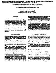
Fig. 4: Illustration of our simple-to-complex strategy for segmentation. Top row (from left to right): input instances, those with ground truth labels, initial clustering output by NCut, and clustering outputs by Gaussian kernel density estimation (KDE) classifiers with σ = 0.35 and 0.1, respectively. Bottom row: refined clustering outputs obtained by our simple-to-complex strategy (i.e., decreasing σ from 0.35 to 0.1). Note that different colors denote the resulting cluster labels.
simple-to-complex strategy effectively performs a coarse-to-fine separation between the observed features. We note that, the use of our simple-to-complex discriminative clustering strategy is to handle objects regions with complex or ambiguous patterns at each image scale. This is very different from existing work like [29,30], which either chose to discriminate between image clusters using predetermined SVMs, and only considered global image statistics for segment discrimination. In our work, the series of classifiers derived by multiple types of features not only make the separation between complex/ambiguous object regions more feasible, the resulting outputs (i.e., clustering results) would also reflect the flexibility of the way human discriminates between different object regions (which is consistent with the observations [31]). In the following subsections, we discuss how we automatically learn the classifiers (or image visual appearance models) with different complexities in each feature space for performing simple-to-complex classification and segmentation. Multiple feature cues Color cues Color information is among the most representative feature cues for image segmentation. As suggested in [14,8], we use CIE Lab color space for representing each image segment, and each channel is represented by a histogram of n bins with equal widths (we set n = 50). Using such features, we apply Naive Bayes classifiers based on kernel density estimation (KDE) [32,25] for separating consecutive image segments. At iteration k of discriminative clustering, we derive the probability distribution of color histograms for each cluster m (i.e., segment label) using Gaussian kernels by: Pck (i|m) ∝
� � � n � X (j − i)2 c h (j) , exp − m σ2 j=1
(1)
Simple-to-Complex Discriminative Clustering for Hierarchical Image Segmentation
7
where c indicates the color channel of interest, and i is the bin index of the associated histogram. From (1), we see that hcm (j) returns the pixel number observed in the jth bin of color channel c, and this number is weighted by a Gaussian kernel with width σ. Note that we do not use the equalityP sign for (1), since the derived probability for each bin will be normalized for ensuring Pck (i|m) = 1. i
As noted in Section 2.2 and depicted in Figure 3, the derivation of (1) can be viewed as the M-step for modeling the cluster information at each iteration in our discriminative clustering process. At the E-step, with the equal prior assumption of the clusters (i.e., same P (m) for each cluster), we classify each image segment s to cluster m (at the E-step) by updating the following probability output: k k PColor (m|s) ∝ PColor (s|m)P (m) =
|s| 3 Y Y
Pck (ip |m),
(2)
p=1 c=1
where ip denotes the bin which the pixel p (in segment s) belongs to, and |s| represents the size of segment s. Similar P kto (1), the calculated probability for each cluster will be normalized for ensuring PColor (m|s) = 1. It is worth noting that, we view each m
pixel as an independent observation for fulfilling Naive Bayes assumptions. Based on our simple-to-complex strategy, we start our KDE-based classification using larger σ values, which perform coarser separation between image segments and alleviate potential overfitting problems. As the iteration continues, we reduce σ (which increases the complexity of KDE) and thus introduce additional classification capabilities based on the separation determined at previous iterations. Texture cues In addition to color, we consider texture information as feature cues for segmentation. As did in [33,34], we also apply 17 Gaussian/Laplacian-type filters and their derivatives in the CIE Lab color space, and we calculate their responses as textural features. In order to describe and summarize such textural responses in each image segment, we perform GMM to construct the textons for computing the associated bagof-words (BoW) models [35,34]. We note that the number of textons would be a tradeoff between the representation and generalization capabilities for the resulting BoW models. While a smaller number of textons produces a simpler/coarser BoW model for describing the texture information, a larger one would exhibit a better representation ability (but more possible for overfitting the texture cues). Therefore, based on our proposed simple-to-complex strategy, we will adjust this parameter during the discriminative clustering process. In our work, we consider 9 different BoW models with different numbers (2 to 32, according to an equal logarithm scale) of textons as discussed below. For the M-stage at iteration k, we estimate the probability distribution of the tth BoW model (t = 1 to 9) for segmentation cluster m. Based on the law of total probability, we calculate Ptk (i|m) as follows: Ptk (i|m) =
X p∈m
P k (i|p)P k (p|m),
(3)
8
Haw-Shiuan Chang and Yu-Chiang Frank Wang
where i is the bin (i.e., texton) index of the tth BoW model, P k (p|m) is that of pixel p presented in cluster m [18], and P k (i|p) calculates the probability of pixel p assigned to bin i (by GMM). At the E-step for re-determining the cluster output for each segment, we need to calculate the probability of assigning each segment s to cluster m (i.e., PTkext (m|s)). Similar to the use of color cues, we define PTkext (m|s) as follows: PTkext (m|s)
∝
Ht 9 Y Y t=1
where P (i|s) =
P
!wt,k P (i|s) Ptk (i|m)
(4)
i=1
P (i|p)P (p|s). Ht indicates the number of textons/bins considered
p
for the tth BoW model (t = 1 ∼ 9), which ranges from 2 to 32 in a descending order. It is worth noting that, wt,k in (4) controls the weight for each BoW model, and it is a function of the iteration number (for simple-to-complex purposes). More specifik cally, we determine wt,k = P (s)exp(−β( kmax − 0.5)t),Pwhere kmax is the maximum iteration number allowed (we set β = 0.1), and P (s) = p P (s|p) is the total number of pixels belonging to segment P s. Similar to (2), the calculated probability of (4) will be normalized for ensuring PTkext (m|s) = 1. It can be seen that we impose a larger m
weight wt,k on BoW models with fewer number of textons (i.e., simpler models) in the beginning stages of our discriminative clustering process. As the iteration increases, a finer separation will be achieved by higher wt,k for the BoW models with larger Ht texton numbers (i.e., finer models). This is how we apply our simple-to-complex strategy for performing textural-based clustering process for segmentation. Locality cues For image segmentation, since the object regions are typically compact and locally connected, spatial information is often considered as another important cue [36,4,5]. In our work, we consider Gaussian and shape prior classifiers. The Gaussian classifiers utilize the x and y coordinates of superpixel centers (extracted at the bottom level in the hierarchy) as features, and thus the observed 2D Gaussian distributions PGk (m|s) can be applied to discriminate between image segments s of different clusters m. On the other hand, inspired by [4], our shape prior classifier aims at deriving the probability P (ps |m) that a superpixel ps is presented at cluster m in terms of its distance to the cluster contour. To be more precise, at the kth iteration of our discriminative clustering process, we derive PSk (ps |m) at the M-step by: ¯ PSk (ps |m) ∝ S(d(ps , m)/d(m)),
(5)
where d(ps , m) measures the shortest distance between superpixel ps to the contour of 1 cluster m. The sigmoid function S(x) = 1+exp(−x) is used to estimate the likelihood of ¯ assigning ps to m, and d(m) is the average distance of d. Assuming the pixels in ps are i.i.d., we estimate the probability of assigning segment s to cluster m as follows: Y |ps | k PShape (m|s) ∝ (PSk (ps |m)) , (6) ps ∈s
Simple-to-Complex Discriminative Clustering for Hierarchical Image Segmentation
9
where |ps | is the size of the superpixel ps . Similar remarks can be applied to the use of Gaussian classifiers. Thus, at the E-step we update the locality cues by fusing the results of the two classifiers by: k k PLocal (m|s) = PGk (m|s)(1−wk ) PShape (m|s)wk ,
(7)
where wk = k/kmax . It can be seen that, as iteration k increases, the weight for the shape prior classifier becomes larger, allowing one to emphasize on object regions with complex shape information (i.e., for finer separation). This is again consistent with our simple-to-complex strategy of the proposed discriminative clustering for segmentation. Graph-based optimization At the E-step of each iteration in our discriminative clustering process, we apply multi-label Markov Random Fields (MRF) for prediction based on the observed feature cues. As discussed later in Section 2.4, this graph-based optimization can be viewed as fitting the observed features of superpixels at the bottom level by the clusters (i.e., image segments) determined at each level in the hierarchy. In our work, we determine the MRF energy term E l (m) at level l as follows: l E l (m) = ED (m) + ESl (m) X l k ED (m) = − wC · log(PColor (ms |s)) + s k wT · log(PTkext (ms |s)) + wL · log(PLocal (ms |s)) X l l ES (m) = λ 1(ms 6=mq ) (−log(PContour (s, q))),
(8)
s,q
where m is the labeling vector indicating the segmentation output, and thus its dimension K is equal to the number of the input segments at that level (i.e., its sth entry ms l indicates the corresponding output for segment s). ED (m) and ESl (m) are the data and l smoothness terms, respectively. While ED (m) integrates the probabilities observed in different feature spaces (with weights wC , wT , and wL ), ESl (m) preserves the consistency of segmentation outputs of neighboring segments. Note that q is the neighboring segments of segment s, and we have ms and mq as cluster labels of segments s and l q, respectively. The function 1() is the indicator function, and PContour (s, q) is the detected contour probability (see Section 2.2). At iteration k in level l of the hierarchy, we apply α-β swap [37,38,39] to minimize (8), and update the cluster label m of each segment s accordingly. With the above MRF model, our discriminative clustering starts segmentation from initial clustering results produced by locally detected contours, and we update the segmentation results at each iteration with increasingly complex classifiers in different feature spaces. 2.4
Probabilistic Interpretation
As discussed above, our simple-to-complex discriminative clustering solves a graphbased optimization problem at each level in the hierarchy, in which each segment is viewed as an input node to be clustered. By increasing the complexities of the MRF energy terms, improved optimization can be achieved. Effectively, at level l, this process
10
Haw-Shiuan Chang and Yu-Chiang Frank Wang 6
3
x 10
Simple only NCut only (w/o DC) w/o hierarchy Complex only Ours
2.8 2.6 2.4 2.2 2 1.8 1.6 1.4 1.2 50
100
150
200
250
300
Fig. 5: Optimized energy function outputs of (8) on BSDS300. The vertical axis is the negative log-likelihood of P l (X) of different approaches, and the horizontal axis indicates the number of clusters determined at each level in our hierarchy. Note that DC denotes discriminative clustering.
is equivalent to the fitting of features observed from superpixels at the bottom level using the clusters determined at level l. For each level l in our hierarchy, minimizing the MRF model in (8) is effectively solving the maximum likelihood estimation (MLE) of probability P l (X): P l (X) =
N Y ps =1
P (xps )
Y
l PContour (ps , pq ),
(9)
ps ,pq
where X represents the observed image features. P (xps ) denotes the estimated probability of superpixel ps at the bottom level, which is observed across K × r differK×r P ent clusters. In other words, we have P (xps ) = P (mps = y)P (xps |mps = y). y=1
The probability term P (mps = y) indicates how likely ps belongs to cluster y, and P (xps |mps = y) is the probability of observing xps in that cluster. For image segmentation, since consecutive superpixels are not independent of each other, we have l PContour (ps , pq ) denote the contour probability of the associated superpixel pair. For our discriminative clustering, each E-step can be viewed as estimating P (mps = y) by minimizing E l in (8), given P (xps |mps = y) observed from the previous Mstep (see the supplementary material for detailed derivations). On the other hand, the M-step at each iteration updates the observed feature models/classifiers, using outputs determined at the E-step. Thus, our simple-to-complex clustering process is effectively solving the above MLE problem. In Figure 5, we show that our discriminative clustering strategy with hierarchical segmentation achieved better and optimized energy function outputs produced at the final iteration in each level, compared with other simplified/controlled versions of our segmentation framework (see our experiments).
3 3.1
Experiments Unsupervised Segmentation
We evaluate our proposed method on the Berkeley Segmentation Datasets (BSDS) [31], MSRC [33], and the Stanford Background Dataset (SBD) [40]. For MSRC, we apply
Simple-to-Complex Discriminative Clustering for Hierarchical Image Segmentation
11
Table 1: Performance comparisons of BSDS (* indicates the methods requiring training data). Note that DC represents discriminative clustering applied in our proposed framework. BSDS300 BSDS500 Methods SegCover PRI VoI SegCover PRI VoI MNCut 0.53 0.79 1.84 0.53 0.80 1.89 SWA 0.55 0.80 1.75 FH 0.58 0.82 1.79 0.57 0.82 1.87 MS 0.58 0.80 1.63 0.58 0.81 1.64 SAS 0.610 0.834 1.534 0.610 0.840 1.552 gPb-OWT-UCM* 0.646 0.852 1.466 0.647 0.856 1.475 ISCRA* 0.66 0.86 1.40 0.66 0.85 1.42 Ours (Full version) 0.660 0.854 1.443 0.655 0.859 1.454 NCut only (w/o DC) 0.583 0.814 1.734 0.578 0.825 1.784 Complex only 0.627 0.840 1.569 0.618 0.845 1.613 Ours w/o MRF 0.633 0.843 1.536 0.634 0.849 1.548 Color cues only 0.595 0.810 1.695 0.598 0.823 1.724 Color + spatial cues 0.605 0.824 1.653 0.605 0.832 1.699
the ground truth labels provided by [41] for evaluation (as [8,16] did). As for SBD, we choose the semantic labels (i.e., “regions” given in [40]) of images as ground truth. We consider three different metrics for evaluating the performance: SegCover [8], PRI [42], and VoI [43]. Note that larger SegCover/PRI and lower VOI numbers indicate better performance. Our code is available at http://mml.citi.sinica.edu.tw/ papers/HDC_code_ACCV_2014/. For our approach, the parameters for BSDS300 are selected based on the performance of the training data of the same dataset. On the other hand, we apply the training data of BSDS500 to determine the parameters for MSRC, SBD, and BSDS500. For evaluation, we perform quantitative evaluations based on the optimal image scale (OIS). That is, the final segment number of interest is determined by the optimal value of each metric based on the ground truth of each image. In order to produce all possible cluster numbers (i.e., other than K at level l, K × r at level l + 1, etc.), we merge the segmentation outputs at that level using the associated contour probability values, so that the intermediate cluster numbers can be obtained. We note that we do not fix the image scale over all images (i.e., optimal dataset scale (ODS)), since unsupervised image segmentation is typically performed prior to higher-level tasks like object recognition or retrieval (e.g. [1,2,3]). For such tasks, image priors of class labels or their semantic information will be provided, which can be viewed as OIS. Later our experiments on semantic segmentation in Section 3.2 will support this observation. Tables 1 and 2 summarize and compare the segmentation results, in which we compare our method with MNCut [10], SWA [17], FH [45], MS (mean shift) [46], SAS [12], gPb-OWT-UCM [8], and ISCRA [16]. From Table 1, it is clear that our approach outperformed baseline approaches. Compared with gPb-OWT-UCM and ISCRA, we achieved comparable or slightly improved results (see examples in Figure 6). As commented in [8], this is due to the fact that inherent photographic bias in BSDS would make images contain sufficient local information, which favors contour-based segmentation
12
Haw-Shiuan Chang and Yu-Chiang Frank Wang
Table 2: Performance comparisons of MSRC and SBD datasets. MSRC SBD Methods SegCover PRI VoI SegCover PRI VoI SAS 0.712 0.823 1.052 0.649 0.856 1.474 gPb-OWT-UCM 0.745 0.850 0.989 0.642 0.858 1.527 ISCRA 0.75 0.85 1.02 0.68* 0.90* 1.50* Ours 0.772 0.862 0.920 0.681 0.870 1.425
Fig. 6: Example segmentation results of BSDS300. From top to bottom: original images, results produced by Mobahi et al. [44], SAS [12], gPb-OWT-UCM [8], and ours. Note that the results for gPb-OWT-UCM, SAS [12] and our method are based on the largest SegCover value, while those of [44] are based on the highest PRI.
approaches like gPb-OWT-UCM or ISCRA. However, it is worth repeating that gPbOWT-UCM and ISCRA applied pre-trained classifiers for contour detection, while ours is an unsupervised approach and does not require the collection of any training data. We note that, if the recently proposed object and part metric of Fop [47] is applied, we achieved a higher score of 0.389 than gPb-OWT-UCM did (0.380). In Table 2, we see that our method achieved the best performance (for ISCRA, we directly apply the results presented in [16], which utilized region-based labels (i.e., “layers” given in [40]) for SBD as ground truth, as noted by * in Table 2). Different from the ground truth of BSDS which separates an object into several regions, image labels for MSRC and SBD are generally able to identify semantical objects [20]. Since our approach is able to observe multiple feature cues for discriminating between image regions, improved performance on these two datasets can be achieved. In addition, we provide controlled experiments in Table 1, which present the contributions of each component in our proposed framework. For example, NCut only represents the use of our hierarchical segmentation framework without performing simple-tocomplex discriminative clustering, and complex only indicates that the use of complex classification models in our proposed method. On the other hand, w/o MRF in Table 1 means the direct use of the predicted probabilities from each feature cue for determining the segmentation outputs (i.e., no smoothness term is considered in (8)).
0.65
0.65
0.6
0.6 SegCover
SegCover
Simple-to-Complex Discriminative Clustering for Hierarchical Image Segmentation
0.55 0.5 0.45 0
Ours Ours gPb gPb−OWT−UCM SAS SAS 5
10 σ
(a) BSDS300
0.55 0.5 0.45
15
13
0.4 0
Ours Ours gPb gPb−OWT−UCM SAS SAS 5
10 σ
15
(b) BSDS500
Fig. 7: Performance comparisons (in SegCover) on degraded versions of BSDS.
To verify that our approach is able to consider non-local information and generalizes well for blurred image contours, we compare the performance our method with those of gPb-OWT-UCM and SAS on BSDS with degraded resolutions. We downgrade the resolution of BSDS300 and BSDS500 images using Gaussian filters with different σ, and we compare the SegCover values in Figure 7. From this figure, we outperformed SAS (region-based) and gPb-OWT-UCM (contour-based) especially when σ is large. Thus, the effectiveness of our approach on lower-resolution images can be verified. 3.2
Semantic Segmentation
We now address the task of semantic segmentation using MSRC and SBD datasets. To be more specific, we evaluate the recognition/annotation accuracy of the output segments, using classifiers learned from training data (with ground truth object label inT GTi S Ri formation) of the corresponding dataset. We apply the metric of ( GTi Ri ) for each semantic class i as recent PASCAL challenges did. Note that GT and R denote the ground truth and detected segments for class i, respectively. A 5-fold cross-validation is conducted. For semantic segmentation, we extract color and texture histograms from ground truth image segments of the training data, and we train classifiers on such image segments using the associated label information (standard Naive Bayes and linear SVM are considered). For the test (validation) images of the same data, we perform image segmentation using our proposed method based on OIS, and we apply the aforementioned classifiers for predicting the class label of each image segment. We compare the performance of ours with SAS and gPb-OWT-UCM. Table 3 compares the averaged results of different approaches. From Table 3, we can see that the average annotation accuracy based on our proposed segmentation method was higher than those using SAS and gPb-OWT-UCM. Note that the optimal performance (denoted as Ground truth in Table 3) was obtained by applying the derived classifiers on the ground truth labeled segments as shown in the last row of Table 3. As a result, we see that our method not only outperformed recent segmentation algorithms in terms of unsupervised segmentation, improved image annotation accuracy also confirms that our approach is able to achieve better semantic segmentation, which would benefit future tasks such as object retrieval and classification.
14
Haw-Shiuan Chang and Yu-Chiang Frank Wang
Table 3: Average recognition results of different methods for semantic segmentation. MSRC SBD Methods Naive Bayes SVM Naive Bayes SAS 0.272 0.330 0.399 gPb-OWT-UCM 0.285 0.352 0.406 Ours 0.294 0.362 0.414 Ground truth 0.366 0.474 0.502
3.3
SVM 0.423 0.426 0.454 0.570
Remarks on Computation Costs
Finally, we comment on the computation time and memory requirements of our proposed method. In average, it took 230 seconds for processing an image in BSDS300 with image resolution around 481 × 321 pixels. The feature processing part (including generating superpixel and building textons) took about 78% of the entire computation time, while our proposed hierarchical segmentation process only required the remaining 22%. Although our method was slightly slower than gPb-OWT-UCM (increased by 5% of the computation time), our method could be easily accelerated if feature extraction or preprocessing steps are performed offline. For example, if we build the textons in advance, our method only took about 60 seconds (only 27% of computation time w.r.t. gPb-OWT-UCM), while the performance only slightly dropped (e.g., SegCover became 0.64 for BSDS500). It is worth noting that, we do not need to solve large-scale eigen-analysis problems as gPb-OWT-UCM does. The memory requirement of our method was about 700MB for each image, which was only 12% of that required by gPb. Note that ISCRA is based on gPb-OWT-UCM and applies more sophisticated features. Therefore, so its memory and computation costs were higher than those of gPb-OWT-UCM. From the above remarks, it can be concluded that our approach is computationally feasible. Note that the above runtime and memory estimates were obtained by Matlab on an Intel Quad Core workstation with 2.2 GHz.
4
Conclusions
This paper presented a hierarchical image segmentation framework, in which an EMbased discriminative clustering is utilized at each level for discriminating between image segments. By our proposed simple-to-complex strategy, a series of classifiers with different generalization capabilities can be learned during the clustering process, so that segmentation of different image segments at each level can be performed automatically. The deployment of our discriminative clustering process in a hierarchical framework allows us to exploit both local and non-local image statistics across image scales when performing unsupervised segmentation. Experimental results on several benchmark datasets confirmed the use of our proposed method for image segmentation, and our method was shown to achieve competitive or improved results than state-of-the-art region or contour-based approaches did.
Simple-to-Complex Discriminative Clustering for Hierarchical Image Segmentation
15
References 1. Pantofaru, C., Schmid, C., Hebert, M.: Object recognition by integrating multiple image segmentations. In: ECCV. (2008) 1, 11 2. Gu, C., Lim, J.J., Arbelaez, P., Malik, J.: Recognition using regions. In: CVPR. (2009) 1, 11 3. Arbelaez, P., Hariharan, B., Gu, C., Gupta, S., Bourdev, L.D., Malik, J.: Semantic segmentation using regions and parts. In: CVPR. (2012) 1, 11 4. Bai, X., Wang, J., Simons, D., Sapiro, G.: Video SnapCut: Robust video object cutout using localized classifiers. In: SIGGRAPH. (2009) 1, 5, 8 5. Papoutsakis, K.E., Argyros, A.A.: Object tracking and segmentation in a closed loop. In: ISVC. (2010) 1, 5, 8 6. Chen, A.Y.C., Corso, J.J.: Temporally consistent multi-class video-object segmentation with the video graph-shifts algorithm. In: WACV. (2011) 1, 5 7. Freixenet, J., Munoz, X., Raba, D., Marti, J., Cufi, X.: Yet another survey on image segmentation: Region and boundary information integration. In: ECCV. (2002) 1 8. Arbelaez, P., Maire, M., Fowlkes, C., Malik, J.: Contour detection and hierarchical image segmentation. IEEE Trans. Pattern Anal. Mach. Intell. (2011) 1, 2, 4, 6, 11, 12 9. Shi, J., Malik, J.: Normalized cuts and image segmentation. In: CVPR. (1997) 1, 4 10. Cour, T., Benezit, F., Shi, J.: Spectral segmentation with multiscale graph decomposition. In: CVPR. (2005) 1, 11 11. Kim, S., Nowozin, S., Kohli, P., Yoo, C.D.: Higher-order correlation clustering for image segmentation. In: NIPS. (2011) 1 12. Li, Z., Wu, X.M., Chang, S.F.: Segmentation using superpixels: A bipartite graph partitioning approach. In: CVPR. (2012) 1, 2, 4, 11, 12 13. Kim, T.H., Lee, K.M., Lee, S.U.: Learning full pairwise affinities for spectral segmentation. IEEE Trans. Pattern Anal. Mach. Intell. (2013) 1 14. Martin, D.R., Fowlkes, C., Malik, J.: Learning to detect natural image boundaries using local brightness, color, and texture cues. IEEE Trans. Pattern Anal. Mach. Intell. (2004) 1, 4, 6 15. Andres, B., Kappes, J.H., Beier, T., Kothe, U., Hamprecht, F.A.: Probabilistic image segmentation with closedness constraints. In: ICCV. (2011) 1, 2 16. Ren, Z., Shakhnarovich, G.: Image segmentation by cascaded region agglomeration. In: CVPR. (2013) 1, 2, 11, 12 17. Sharon, E., Galun, M., Sharon, D., Basri, R., Brandt, A.: Hierarchy and adaptivity in segmenting visual scenes. In: Nature. (2006) 2, 11 18. Alpert, S., Galun, M., Basri, R., Brandt, A.: Image segmentation by probabilistic bottom-up aggregation and cue integration. In: CVPR. (2007) 2, 8 19. Fowlkes, C.C., Martin, D.R., Malik, J.: Local figure–ground cues are valid for natural images. Journal of Vision (2007) 2 20. Zitnick, C.L., Parikh, D.: The role of image understanding in contour detection. In: CVPR. (2012) 2, 12 21. Levinshtein, A., Stere, A., Kutulakos, K.N., Fleet, D.J., Dickinson, S.J., Siddiqi, K.: Turbopixels: Fast superpixels using geometric flows. IEEE Trans. Pattern Anal. Mach. Intell. (2009) 3 22. Pele, O., Werman, M.: A linear time histogram metric for improved sift matching. In: ECCV. (2008) 4 23. Pele, O., Werman, M.: Fast and robust earth mover’s distances. In: ICCV. (2009) 4 24. Rother, C., Kolmogorov, V., Blake, A.: ”GrabCut”: interactive foreground extraction using iterated graph cuts. SIGGRAPH (2004) 5 25. Pham, V.Q., Takahashi, K., Naemura, T.: Foreground-background segmentation using iterated distribution matching. In: CVPR. (2011) 5, 6
16
Haw-Shiuan Chang and Yu-Chiang Frank Wang
26. Zhu, S.C., Yuille, A.L.: Region competition: Unifying snakes, region growing, and bayes/mdl for multiband image segmentation. IEEE Trans. Pattern Anal. Mach. Intell. (1996) 5 27. Belongie, S., Carson, C., Greenspan, H., Malik, J.: Color-and texture-based image segmentation using EM and its application to content-based image retrieval. In: Computer Vision. (1998) 5 28. Achanta, R., Shaji, A., Smith, K., Lucchi, A., Fua, P., Ssstrunk, S.: SLIC superpixels compared to state-of-the-art superpixel methods. IEEE Trans. Pattern Anal. Mach. Intell. (2012) 5 29. Xu, L., Neufeld, J., Larson, B., Schuurmans, D.: Maximum margin clustering. In: NIPS. (2004) 6 30. Gomes, R., Krause, A., Perona, P.: Discriminative clustering by regularized information maximization. In: NIPS. (2010) 6 31. Martin, D.R., Fowlkes, C., Tal, D., Malik, J.: A database of human segmented natural images and its application to evaluating segmentation algorithms and measuring ecological statistics. In: ICCV. (2001) 6, 10 32. Witten, I., Frank, E., Hall, M.: Data Mining: Practical Machine Learning Tools and Techniques. Morgan Kaufmann, San Francisco (2005) 6 33. Shotton, J., Winn, J., Rother, C., Criminisi, A.: Textonboost: Joint appearance, shape and context modeling for multi-class object recognition and segmentation. In: ECCV. (2006) 7, 10 34. Yu, Z., Li, A., Au, O.C., Xu, C.: Bag of textons for image segmentation via soft clustering and convex shift. In: CVPR. (2012) 7 35. Calinon, S., Guenter, F., Billard, A.: On learning, representing and generalizing a task in a humanoid robot. IEEE Transactions on Systems, Man and Cybernetics, Part B. Special issue on robot learning by observation, demonstration and imitation (2007) 7 36. Carreira, J., Sminchisescu, C.: Constrained parametric min-cuts for automatic object segmentation. In: CVPR. (2010) 8 37. Boykov, Y., Veksler, O., Zabih, R.: Fast approximate energy minimization via graph cuts. IEEE Trans. Pattern Anal. Mach. Intell. (2001) 9 38. Kolmogorov, V., Zabih, R.: What energy functions can be minimized via graph cuts? IEEE Trans. Pattern Anal. Mach. Intell. (2004) 9 39. Boykov, Y., Kolmogorov, V.: An experimental comparison of min-cut/max-flow algorithms for energy minimization in vision. IEEE Trans. Pattern Anal. Mach. Intell. (2004) 9 40. Gould, S., Fulton, R., Koller, D.: Decomposing a scene into geometric and semantically consistent regions. In: ICCV. (2009) 10, 11, 12 41. Malisiewicz, T., Efros, A.A.: Improving spatial support for objects via multiple segmentations. In: BMVC. (2007) 11 42. Unnikrishnan, R., Pantofaru, C., Hebert, M.: Toward objective evaluation of image segmentation algorithms. IEEE Trans. Pattern Anal. Mach. Intell. (2007) 11 43. Meila, M.: Comparing clusterings: an axiomatic view. In: ICML. (2005) 11 44. Mobahi, H., Rao, S., Yang, A.Y., Sastry, S.S., Ma, Y.: Segmentation of natural images by texture and boundary compression. IJCV (2011) 12 45. Felzenszwalb, P.F., Huttenlocher, D.P.: Efficient graph-based image segmentation. IJCV (2004) 11 46. Comaniciu, D., Meer, P.: Mean shift: A robust approach toward feature space analysis. IEEE Trans. Pattern Anal. Mach. Intell. (2002) 11 47. Pont-Tuset, J., Marqus, F.: Measures and meta-measures for the supervised evaluation of image segmentation. In: CVPR. (2013) 12