Sadiq M. Sait, Aiman H. El-Maleh, and Raslan H. Al-Abaji. King Fahd University ..... [7] Junaid A. Khan, Sadiq M. Sait, and Mahmood R. Minhas. Fuzzy Biasless ...
SIMULATED EVOLUTION ALGORITHM FOR MULTIOBJECTIVE VLSI NETLIST BI-PARTITIONING Sadiq M. Sait, Aiman H. El-Maleh, and Raslan H. Al-Abaji King Fahd University of Petroleum & Minerals Computer Engineering Department Dhahran 31261, Saudi Arabia sadiq,aimane,raslan�@ccse.kfupm.edu.sa ABSTRACT In this paper, the Simulated Evolution algorithm (SimE) is engineered to solve the optimization problem of multi-objective VLSI netlist bi-partitioning. The multi-objective version of the problem is addressed in which, power dissipation, timing performance, as well as cut-set are optimized while Balance is taken as a constraint. Fuzzy rules are used in order to design the overall multiobjective cost function that integrates the costs of three objectives in a single overall cost value. Fuzzy goodness functions are designed for delay and power, and proved efficient. A series of experiments are performed to evaluate the efficiency of the algorithm. ISCAS-85/89 benchmark circuits are used and experimental results are reported and compared to earlier algorithms like GA and TS. 1. INTRODUCTION VLSI circuit design has various objectives. Until the beginning of this decade, two main objectives of VLSI circuit design were: the minimization of interconnect wire length and the improvement of timing performance. A large number of efforts targeting either one (especially cut-set) or both of the above objectives are reported in the literature[1, 2]. The power consumption of the circuit was not of main concern while trying to optimize the above two objectives. As different techniques are applicable and have been reported [3] at different steps of the VLSI design process, few performance-driven partitioning techniques at physical level design exist in literature. Furthermore, to our knowledge, no effort has been reported that targets the optimization of three objectives simultaneously (power, delay, cut-set). In this work, the above problem is addressed in the partitioning step at the physical level. The Simulated Evolution algorithm is tailored for the multiobjective optimization of Partitioning. This paper is organized as follows. In the next section, the SimE algorithm is introduced. In Section 3 the problem is presented and the cost functions are formulated. Section 4 presents the goodness functions and the design implementation details of the algorithm, and then experimental results are reported and discussed in section 5. 2. SIME ALGORITHM In this section, Simulated Evolution is summarized. The pseudocode of SimE is given in [4]. SimE operates on a single solution, termed as � �������. Each population consists of elements. In case of partitioning problem, these elements are cells to be moved. In the Evaluation step, goodness of each element is measured. Goodness of an element is a single number between ‘0’ and ‘1’, which is a measure of how near is the element from its optimal
location. After that comes Selection which is the process of selecting those individuals which are unfit (badly placed) in the current solution. For that purpose, goodness of each individual is compared with a random number (in the range [0,1]), if the goodness is less than the random number then it is selected. The whole algorithm is repeated until some stopping criteria is met. Stopping criteria may be the number of iterations for which there is no further improvement in the overall cost, or total number of iterations are completed. At the end of Repeat loop, the algorithm returns the best solution found. Higher value of goodness means that the element is near its optimal location. For SOP, the goodness can be calculated as follows, � �
(1)
ALGORITHM ������� � ���� �� � � � � � = Bias Value. � = Complete Solution. � = Initial Solution. � = Stopping Criterion. � = Individual link in �. � = Lower bound on cost of ��� link. � = Current cost of ��� link in �. � = Goodness of ��� link in �. = Queue to store the selected links. ��� ���� � � � � allocates � in partial solution � . Repeat EVALUATION:
SELECTION:
ALLOCATION:
ForEach � � DO Begin Evaluate � End ForEach � � DO Begin If ����� � � �� Begin
��; � ��� ; End End sort � ForEach � DO Begin End
��� ���� � � �
�
�� �
�
Until SC is satisfied Return (Best solution) End ������� � ����
Figure 1: Structure of the simulated evolution algorithm. In Selection, an individual having high goodness measure still has a non-zero probability of assignment to set � . It is this element of non-determinism that gives SimE the capability of escaping local minima. After the selection process, the allocation
μ ci
operator is used to place cells in � to new locations. The choice of allocation function is problem specific.
μ c width 1.0
1.0
3. PROBLEM FORMULATION AND COST FUNCTIONS This work addresses the problem of VLSI netlist partitioning with the objectives of optimizing power consumption, timing performance (delay), and cut-set while considering the Balance constraint (same as area constraint as unit area is assumed for every gate). Formally, the problem can be stated as follows: � ��
�� �, the purpose of Given a set of modules
partitioning is to assign the modules to a specified number of clusters � (two in our case) satisfying prescribed properties. In general, a circuit can have multi-pin connections (nets) apart from two-pin. Our task is to divide into subsets (blocks) � and in such a way that the objectives are optimized, subject to some constraints.
�
Cutsize The cutsize cost function can be also be written as follows : � � �
�������
(2)
¾ where � � � denotes the set of off-chip wires. The weight ���� on the edge � represents the cost of wiring the corresponding connection as an external wire. � �
�� ��
Delay In the general delay model where gate delay � � and constant inter-chip wire delay are considered, �� � � � where �� is actually due to the off-chip capacitance denoted as ��� � . Let the delay of node � � be � � and the delay of net � � � which is cut be �� . Given a partition
� , the path delay � between nodes � and � is the sum of the node delays � � � and the delay of nets which are cut, that is :
� �
��� � �
� � � � � �
������� �
�
� �
¾�
��
� � �
�����
�
�
(3)
�
� �
��� �
� ���
�
��
�
(4)
where � ��� is the load capacitance, �� is the supply voltage, ���� � is the global clock period, and � is the number of gate output transitions per clock cycle. � is calculated using the symbolic simulation technique of [5] under a zero delay model. � ��� in Eq. 4 consists of two components: ���� � which accounts for the load capacitances driven by a gate before circuit partitioning, and the extra load � ����� which accounts for the additional load capacitance due to the external connections of the net after circuit partitioning. Then, the total power dissipation of any circuit � is: ��
�
� � �� ���
¾�
�� � � � � � ��� ��
(5)
where � is a constant that depends on technology. When a circuit partitioning corresponds to a physical partitioning, ������ of a gate that is driving an external net is much larger than ���� � . Area or Balance Constraint The balance constraint is given as follows:
��� � �� � � � �
(6)
C width /O width
C i/O i
gi
g width
(a)
(b)
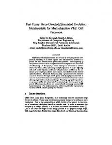
Figure 2: Membership function(s). where � is the number of cells in partition � and � is the total number of cells in the circuit, and the balance factor � � �� .
��
��
3.1. Overall Fuzzy Cost Function: In order to solve the multiobjective partitioning problem, linguistic variables are defined as: cut-set, power dissipation, delay and balance. The following fuzzy rule is used to combine the conflicting objectives IF a solution has Small cut-set AND Low power consumption AND Short delay AND Good Balance THEN it is an GOOD solution. The above rule is translated to and-like OWA fuzzy operator [6] and the membership � � of a solution � in fuzzy set good solution is given as:
��
��� �� ���
��
������� ���� �� ���� ��� ���� ��� ���� �
�� � �� � ��
� ��
Power The average dynamic power consumed by a CMOS logic gate in a synchronous circuit is given by: �� ��
g i*
1.0
��
��� ���
(7)
���� ����
where �� � is the membership of solution � in fuzzy set of acceptable solutions, ������ � is the membership value in the fuzzy sets of “ within acceptable power”, “within acceptable delay”, “within acceptable cut-set” and “within acceptable balance” respectively. � � is the constant in the range , the superscript � represents the cost. In this paper, �� � is used as the aggregating function. The solution that results in maximum value of �� � is reported as the best solution found by the search heuristic. The membership functions for fuzzy sets Low power consumption, Short delay, Small cut-set, are shown in Fig. 2(a) We can vary the preference of an objective � in the overall membership function by changing the value of which represents the relative acceptable limits for each objective whrere � . Fig. 2(b) represents the membership functions for fuzzy set good Balance. ! is the estimate of lower bound on the cost of an individual �, and � is the actual cost of �. ! ’s are independent of iteration, therefore, these are estimated only in the beginning. Whereas, � has to be calculated in every iteration for every element.
��
��
��
��
�
4. PROPOSED SCHEME AND IMPLEMENTATION DETAILS In this section, several important implementation details of SimE algorithm are discussed. The description is combined with fuzzy
logic implementation. In the proposed algorithm, interconnect power dissipation, overall circuit delay and Cutset are used as objectives and Balance as a constraint, which makes it a MOP. In order to solve this MOP, fuzzy logic that provides a convenient method to combine possibly conflicting objectives is used. It is clear that fuzzy logic can be applied at different stages of the SimE algorithm. These stages are evaluation and allocation. In the proposed algorithm, fuzzy logic is applied to the evaluation stage. In the evaluation stage, a new strategy for evaluating the goodness of a cell is employed.
Partition 1
;;
�
0.3
��
��
�
�
of a cell is defined as a Power Goodness The power goodness measure of how well placed is the cell in its present block according to power consumption and can be computed as follows:
�
�
�� �� ��� �
� � � � ���� �� �� � � �� �� � � � ���
�
�
(9)
$ is the switching probability of the cell that drives the net. The goodness is equal to the sum of the switching probabilities of the cells that are driving the uncut nets over the sum of the switching probabilities of the cells that are driving all nets connected. In this way a cell is placed in the partition where the sum of the switching probability of the cut nets is optimized. Results show that this goodness function gives high quality solutions with less power dissipation. Since � � we can take the fuzzy membership �� . An example of power goodness calculation is shown in Fig. 3; the goodness of cell is calculated as ��� ���
. follows: �� ��� The power and cutset objectives are possibly conflicting. Hence it is possible to find alternative solutions for a specific circuit. For example, there may exist a solution with high number of cuts and low power consumption (because the nets cut have less switching probability) and another with lower cuts and higher power consumption. Delay Goodness In our problem, we deal with multi-pin nets, which makes it hard to design a suitable and simple delay goodness function. We propose the following delay goodness.
�
� ���
2
0.1 6
0.4
Figure 3: Power and Cut Goodness Calculation.
;; ;;;; ; ;; Partition 1
D
SET
Partition 2 3
Q
1
CLR
Q
4
2
5
7
6
D
SET
CLR
where � is the goodness of cell �,
� ��
� � is the set of nets connected to cell �, " is a subset of containing the connected nets to cell � that are cut; the cardinality of is expressed as � . The net � is said to be cut if and only if cell � � � and cell � � � and #���� � � #���� � . The number of nets connected to � and having the status as cut is expressed as � . The cut goodness is simply the number of uncut nets over the total nets connected. Since � is between and , we can take the fuzzy membership �� as equal to the goodness �� � . An example of goodness calculation is shown in Fig. 3; the goodness of cell � � is calculated as follows: ��
. �
�
0.2
5
7
(8)
4
0.2
In this stage of the algorithm, goodness of individual cell is computed. �, and � are defined to be Delay, power and cut goodness of a cell, respectively. A fuzzy membership for each goodness function is then derived in order to get the overall goodness of the cell in its partition. Cut Goodness Taking into account the hypergraph representation of the circuit, the goodness function � is defined and computed as follows:
��
3
1
4.1. Proposed Fuzzy goodness Evaluation Scheme
Partition 2
0.1
� � � �! � � �
(10)
Q
Q
Figure 4: Delay Goodness Calculation. where � is the delay goodness of cell �. We consider the set of all critical paths passing through � and define the set % as the set of all cells connected to these paths. We also define & as a subset of % , containing those cells which are connected to all critical paths passing through � and are not in the same block as �. This goodness function will tend to drive the cells that are connected by the critical path to the same block, thus minimizing the delay along the path. A cell is considered good in its block if the majority of cells connected to all critical paths passing through it are also placed in the block. An example for delay computation is given for the in Fig. 4. To calculate �� , we first compute %� critical path 1,4,5,7,6� which is the only one connected to cell . � � &� which are cells �. This gives ��
. �
, and hence is better placed according to the However, �� delay consideration.
��
�
� ��
4.2. Proposed Fuzzy Evaluation Scheme and Selection With the classical goodness of cut only, it is possible that a cell having a high goodness with respect to cut may not be selected even though it is badly placed with respect to circuit delay and power. In order to overcome this problem, it is necessary to include power and delay in the goodness measure along with cut goodness. Also, it is not desirable to select all the cells even if they all have a low goodness value. In this case, it is desirable to select those cells which are far from their lower bounds as compared to other cells in the design. For this purpose, the following fuzzy rule is proposed. Rule R1: (as compared to other cells) IF cell � is near its optimal Cut-set goodness AND near its optimal power goodness AND near its optimal net delay goodness OR �� � � is much smaller than �� � THEN it has a high goodness.
��
Circuit S298 S386 S641 S832 S953 S1196 S1238 S1488 S1494 S2081 S3330 S5378 S9234 S13207 S15850
D (ps) 197 393 886 400 476 415 350 612 502 325 394 554 831 1014 1189
Simulated Evolution SimE Cut P(sp) � �� Best(s) 11 837 0.95 62 28 1696 0.74 152 16 1738 0.98 966 39 3132 0.691 257 48 2473 0.93 249 78 5488 0.82 398 77 5960 0.73 205 83 5892 0.7 716 71 6250 0.81 802 13 706 0.94 89 46 8431 0.98 812 161 14094 0.95 465 196 25672 0.98 3853 313 35014 0.98 3129 416 40716 0.96 1850
D (ps) 233 356 1043 444 526 396 475 571 614 302 571 587 1313 1399 1820
Genetic Algorithm Cut P(sp) � �� 19 1013 0.79 36 1529 0.75 45 2355 0.83 45 3034 0.68 96 2916 0.69 123 5443 0.76 127 5713 0.72 104 5648 0.71 102 5474 0.70 26 787 0.73 299 10358 0.75 573 18437 0.74 1090 38149 0.72 1683 45611 0.74 2183 51747 0.74
Best(s) 43 151 1540 276 182 373 365 1183 1040 32 2074 2686 5949 8097 10206
D (ps) 197 386 889 446 466 301 408 528 585 225 533 590 1052 843 1411
Cut 24 30 59 50 99 106 79 98 101 17 295 430 918 1332 1671
Tabu Search P(sp) � �� 926 0.81 1426 0.76 2281 0.85 2731 0.682 2518 0.734 4920 0.801 4597 0.75 5529 0.72 5339 0.71 770 0.79 10298 0.79 16527 0.79 34055 0.81 41114 0.79 47480 0.831
Best(s) 21 77 818 80 225 134 160 405 427 16 994 1100 2821 3690 5130
Table 1: Comparison between SimE, GA and TS
1.0
1
Tmax(i) is much smaller than Tmax
μ epath
0.9
1.0
X
2.0
e path
��
Figure 5: Membership function for ���� � ���� . Where ���� is the delay of the most critical path in the current iteration and ���� � is the delay of the longest path traversing cell � in the current iteration. The membership function is illustrated in Fig. 5. In our implementation, the Biasless Selection scheme proposed by Khan et al in [7] is used. The selection bias # is totally eliminated and a cell is selected if '����( ) �����** .
��
5. EXPERIMENTAL RESULTS Table 1 present the results obtained from running the SimE, GA, and TS (implementation details in [8]). Results suggest that the quality of solutions obtained by SimE outperformed both GA and TS in terms of quality of solution and time of execution.Fig. 6 shows the performance of SimE versus TS and GA with respect to time, it can be seen clearly that SimE outperforms both algorithm, in quality and runtime. 6. CONCLUSIONS In this paper, the SimE iterative algorithm for multiobjective VLSI Partitioning is proposed. For that purpose goodness functions for delay and power are designed. Fuzzy logic was used in two levels for the final cost function as well as the final goodness funtion. It is used to integrate three objectives namely power, delay, and cutset into a scalar cost value. It is observed that SimE out performs GA and TS in terms of final solution costs and execution time. Acknowledgment: The authors thank King Fahd University of Petroleum & Minerals, Dhahran, Saudi Arabia, for support, under project #:COE/ITERATE/221 7. REFERENCES [1] Sadiq M. Sait and Habib Youssef. VLSI Physical Design Automation: Theory and Practice. McGraw-Hill Book Company,
Maximum Fitness per generation
0.8
0.7
0.6
0.5
0.4
0.3
0.2
TS GA SimE 0
1000
2000
3000
4000 5000 Generations
6000
7000
8000
9000
Figure 6: Multi objective SimE, GA and Ts performance for the circuit S13207 against time. Europe, 1995. [2] K. Shahookar and P. Mazumder. VLSI Cell Placement Techniques. ACM Computing Surveys, 2(23):143–220, June 1991. [3] M. Pedram. CAD for Low Power: Status and Promising Directions. IEEE International Symposium on VLSI Technology, Systems and Applications, pages 331–336, 1995. [4] Sadiq M. Sait and Habib Youssef. Iterrative Computer Algorithms with Applications in Engineering: Solving Combinatorial Optimization Problems. IEEE Computer Society Press, California, December 1999. [5] A. Ghosh, S. Devadas, K. Keutzer, and J. White. Estimation of Average Switching Activity in Combinational and Sequential Circuits. Design Automation Conference, pages 253–259, 1992. [6] R. R. Yager. On Ordered Weighted Averaging Aggregation Operators in Multicriteria Decisionmaking. IEEE Transaction on Systems, MAN, and Cybernetics, 18(1), January 1988. [7] Junaid A. Khan, Sadiq M. Sait, and Mahmood R. Minhas. Fuzzy Biasless Simulated Evolution for Multiobjective VLSI Placement. IEEE CEC 2002, Hawaii USA, 12-17 May 2002. [8] R. H. Al-Abaji. Evolutionary Techniques for Multi-objective VLSI Netlist Partitioning. Master’s thesis, King Fahd University of Petroleum and Minerals, Dhahran, Kingdom of Saudi Arabia, May 2002.