A Simulated Annealing Algorithm for Makespan

ANEXO 1: ARTÍCULO DE INVESTIGACIÓN

A Simulated Annealing Algorithm for Makespan Minimization on Nonidentical Batch Processing Machines Mario C. Vélez-Gallego Departamento de Ingeniería de Producción Universidad EAFIT. Medellín, Colombia José A. Montoya Departamento de Ingeniería de Producción Universidad EAFIT. Medellín, Colombia

Purushothaman Damodaran Department of Industrial & Systems Engineering Florida International University, Miami, FL 33174 Abstract A simulated annealing approach is proposed to minimize the makespan on a set of non-identical batch processing machines arranged in parallel. The scheduling problem under study has the following characteristics: arbitrary job sizes, arbitrary job processing times, and non-identical machine capacities. Each machine can process several jobs simultaneously as a batch as long as the machine capacity is not violated. The batch processing time is equal to the largest processing time among those jobs in the batch. The performance of the proposed solution approach (both in terms of solution quality and run time) are evaluated by solving random problem instances and comparing the results to a solution approach reported in the literature. The experimental study indicates that the proposed solution approach outperforms the existing method.

Keywords Batch processing machines, makespan, simulated annealing

1. Introduction In electronics manufacturing, Printed Circuit Boards (PCBs) go over a series of processes and at the end of which they are tested on environmental stress screening (ESS) chambers. ESS chambers can process several PCB´s simultaneously as a batch, as long as the total size of the PCBs in the batch does not violate the chamber’s capacity. In the process that motivated this work, PCBs from different production lines arrive dynamically to a queue in front of a set of ESS chambers where they are grouped into batches for further testing. The capacities of the ESS

32

chambers are not necessarily identical. Each line delivers PCBs that vary in size and require different processing times at the chamber. Once a batch is formed, its processing time is the longest processing time among the PCBs in the batch. ESS chambers are expensive and a bottleneck. Consequently, manufacturers are interested in maximizing their utilization (i.e. minimizing the makespan). For the remainder of this paper PCBs will be referred to as jobs and ESS chambers as batch processing machines. The problem can be formally stated as follows: the objective is to minimize the makespan (Cmax) on the set {m ∈ M} of batch processing machines arranged in parallel, each with capacity Sm. A set {j ∈ J} of n jobs are to be processed on any one of the given machines. The processing time pj and the size sj of each job j are given. The total size of all the jobs in a batch assigned to machine m should not exceed Sm (i.e. machine capacity). The decisions to make are to (1) group jobs into batches, and (2) schedule the batches formed so that the makespan is minimized. Using the α | β | γ notation introduced by Graham et al. [1], the problem under study can be represented as Rm | batch | Cmax. The problem is NP–hard. When Sm = S ∀ m ∈ M, and sj = S ∀ j ∈ J the problem under study reduces to the classical Pm || Cmax, problem, which is NP- hard [2]. The objective of this research is to develop a Simulated Annealing (SA) algorithm for the problem under study and evaluate its performance in terms of solution quality and run time.

2. Previous Related Work Makespan minimization has been addressed by several researchers under the assumption of parallel batch processing machines of identical capacity: Chang et al. [3] proposed a SA approach, Koh et al. [4] assumed incompatible job families with a common family processing time and proposed several heuristics and a Genetic Algorithm (GA), Kashan et al. [5] developed a GA, and Shao et al. [6] proposed a neural network approach. The problem of makespan minimization on identical batch processing machines under non-zero job ready times has been addressed by Chung et al [7] who extended the DELAY heuristic proposed by Lee and Uzsoy [8] for the single machine case. Damodaran and Velez–Gallego [9] proposed several heuristics for the same problem. To the best of our knowledge, the only research effort that addresses the problem under study is that of Xu and Bean [10] who developed a GA approach using the so-called random keys encoding. The aim of this work is to propose a SA approach and evaluate the solution quality by comparing the results with the approach proposed by Xu and Bean. Introduced by Kirkpatrick et al. [11] and Cerny [12], the metaheuristic known as simulated annealing (SA) is probably the most widely used metaheuristic in combinatorial optimization. It was motivated by the analogy between the physical annealing of metals and the process of searching for the optimal solution in a combinatorial optimization problem. SA is a randomized local search heuristic that, in a minimization problem, allows for uphill movements in order to prevent the algorithm from getting trapped at local optima. It has been successfully applied to solve a variety of combinatorial optimization problems including the traveling salesman and the quadratic assignment problem, graph coloring and partitioning, production scheduling, vehicle routing, and many others. We refer to [13, 14] for extensive surveys on applications of SA to solve complex combinatorial problems. A detailed explanation of the algorithm can be found in [15].

3. Solution Approach The initial solution required to start the algorithm is constructed as follows: (1) the jobs are assigned to the machines at random, (2) following the order in which the jobs were assigned to each machine the batches are formed such that the machine capacity is not violated, and (3) the makespan of the resulting schedule was

33

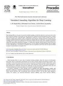
calculated. We use the 10-job problem instance presented in Table 1 to illustrate how the initial solution is obtained. Suppose that two batch processing machines are available with capacities S1=7 and S2=5. The initial solution is constructed as follows: we randomly assign jobs 1, 2, 5, and 9 to machine 1, and jobs 3, 4, 6, 7, 8 and 10 to machine 2. Following the order of the assignment we form batches {1, 2, 5} and {9} in machine 1 with processing times 7 and 9 respectively, and batches {3, 4}, {6, 7} and {8, 10} with processing times 10, 9 and 4. The resulting makespan is 23. A Gantt chart of the resulting schedule is shown in Figure 1.

j pj sj

1 7 1

2 6 3

Table 1: 10-job problem instance 3 4 5 6 7 10 7 5 3 9 1 3 3 2 3

8 4 1

9 9 3

10 4 2

Figure 1: Gantt chart of the initial solution The SA algorithm generates new solutions in the neighborhood of the current solution by two mechanisms: job interchanges and job insertions. In the first mechanism, two jobs assigned to different batches in the current schedule are interchanged; in the second, one job is moved from one batch to another. The batch(es) are chosen at random for the interchange and exchange mechanisms. While interchanging and exchanging jobs the capacity of the machine should not be exceeded. The neighboring solution is obtained after performing a job interchange with probability θ, or a job insertion with probability 1 – θ. Figures 2 and 3 illustrate examples of a job interchange and a job insertion respectively on the initial solution explained before.

Figure 2: Example of a job interchange

34

Figure 3: Example of a job insertion T0, the initial value of the parameter T known as the temperature, is chosen so that at the early stages of the search process, the neighboring solutions are accepted with a high probability φ ≈ 1. To do this, we first explore the proposed neighborhood around the initial solution for a fixed number of times (i.e. 20). The best and worst objective function values are kept as Cmax(best) and Cmax(worst), and T0 is obtained by solving equation (1) for T with φ = 0.9.

At each value of T the algorithm evaluates a fixed number of N neighboring solutions, where N is calculated as a function of the problem size (i.e. N = α.n). A neighboring solution is accepted if its makespan, Cmax(neighbor), is less than the makespan of the current solution Cmax(current); if not, the algorithm generates a uniform random number w over (0,1), and accepts the new non–improving solution if w ≤ q, where q is evaluated as in equation (2). The cooling rate ε is a real–valued parameter between 0 and 1 such that the value of T at iteration k+1, Tk+1 is calculated as Tk+1=ε∙Tk. To stop the algorithm a counter is incremented every time a new neighboring solution is evaluated, and is set to zero when the best solution is updated. The algorithm stops if the counter reaches the value of MaxStopCount, which is calculated as a linear function of the problem size as MaxStopCount = β∙n.

Let α, β, ε and θ be the parameters in the algorithm. Let x be a feasible schedule of the problem under study, and Interchange(x) and Insertion(x) be the functions that perform a feasible interchange and a feasible insertion over x, respectively. Cmax(x) returns the makespan of the feasible schedule x and Neighbor(x, θ) returns a feasible schedule in the neighborhood of x as follows:

35

y = Neighbor (x, θ) y←x Generate z ~ U[0, 1] if z ≤ θ then y = Interchange(y) else y = Insertion(y) end if The proposed simulated annealing algorithm is the following: begin Make T ← T0, k ← 0, count ← 0 Let x be the initial solution to the problem Make xbest ← x, xcurrent ← x while count ≤ β∙n for i =1 to α∙n xnew ← Neighbor (xcurrent, θ) count ← count + 1 if Cmax(xnew) ≤ Cmax(xcurrent) then xcurrent ← xnew count ← 0 if Cmax(xcurrent) ≤ Cmax(xbest) then xbest ← xcurrent end if else Generate w ~ U[0, 1] Compute q (as in equation 2) if w ≤ q then current new x ←x end if end if end for T ← ε∙T end while end The experimental study conducted to evaluate the performance of the proposed SA approach is presented in the following section.

36

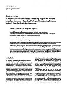
4. Experimental Results The proposed SA algorithm was evaluated by comparing its results to the Random Keys Genetic Algorithm (RKGA) published in [10]. To make this comparison random problem instances were generated following the procedure described in [10] as follows: three problem sizes (i.e. 15, 50 and 100 jobs) and two machine settings (i.e. 2 and 4 machines) were considered. For each combination of problem size and machine setting, 10 random instances were generated, for a total of 60 instances. The processing times were sampled from a discrete uniform distribution between 1 and 10 (DU[1, 10]). For each set of 10 instances, the job sizes of the first five were generated from DU[1, 4] and the job sizes of the remaining five were generated from DU[2, 8]. Finally, for each machine setting, the machine capacities were generated from DU[8, 12]. Table 1 summarizes the factors and levels used to generate the problem instances. Both the SA and RKGA were coded in MatLab 7.1 and run on a desktop computer with a 1.86 GHz Quad Core processor and 4 GB of RAM. Table 2: Instance generation factors and levels Factors Levels Values Number of jobs, |J| 3 15, 50, 100 Processing time, pj 1 DU[1, 10] Job size, sj 2 DU[1, 4], DU[2, 8] Number of machines, |M| 2 2, 4 Machine capacity, Sm 1 DU[8, 12] Each problem instance was solved 5 times using both approaches and relevant statistics were collected. As in [10], the medians were used instead of the average makespan to reduce the influence of extreme values. The percentage of makespan improvement of the SA over the RKGA was calculated as in equation (3). Figure 4 presents the average percentage of makespan improvement.

Figure 4: Makespan Improvement

37

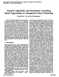
From the analysis it can be concluded that the SA outperformed RKGA with respect to solution quality. The analysis also showed that the average improvement is higher when the job size distribution is DU[2, 8]. A similar analysis was conducted to compare the computational (run) times of both RKGA and SA. For each problem instance the average run time required over 5 independent runs was recorded. The improvement of the SA over the RKGA approach with this respect was calculated as in equation (4). Figure 5 shows the average improvement in run time.

Figure 5: CPU Time or Run-Time Improvement

5. Conclusion Rm|batch|Cmax is an NP-Hard problem. Consequently a simulated annealing approach was proposed to solve the problem within reasonable computational time. The performance of the proposed simulated annealing (SA) algorithm was compared to a genetic algorithm (GA) approach published in the literature with respect to solution quality and computational cost. On average, the proposed SA approach found solutions 4.7% better than the GA. The computational time of the SA algorithm was on average 80.4% less than GA.

References 1. 2. 3. 4. 5. 6.

Graham, R. L., Lawler, E. L., Lenstra, L. K., and Rinnooy Kan, A. H. G., 1979, “Optimization and approximation in deterministic sequencing and scheduling: a survey”, Annals of Discrete Mathematics, 5, 287-326. Garey, M. R. and Johnson, D. S., 1979, Computers and intractability a guide to the theory of NP-completeness, W. H. Freeman, San Francisco. Chang, P.-Y., Damodaran. P., and Melouk, S., 2004, “Minimizing makespan on parallel batch processing machines”, International Journal of Production Research, 42(19), 4211-4220. Koh, S.-G., Koo, P.-H., Kim, D.-C., and Hur, W.-S., “Scheduling parallel batch processing machines with arbitrary job sizes and incompatible job families”, International Journal of Production Economics, 98(1), 81-96. Kashan, A. H., Karimi, B., and Jenabi, M., 2008, “A hybrid genetic heuristic for scheduling parallel batch processing machines with arbitrary job sizes”, Computers and Operations Research, 35(4), 1084-1098. Shao, H., Chen, H.-P., Huang, G. Q., Xu, R., Cheng, B.-Y., Wang, S.-S., and Liu, B.-W., 2008, “Minimizing makespan for parallel batch processing machines with non-identical job sizes using neural nets approach”,

38

Proc. of the 3rd IEEE Conference on Industrial Electronics and Applications (ICEIA), June 3-5, Singapore, 19211924. 7. Chung, S. H., Tai, Y. T., and Pearn, W. L., 2008, “Minimising makespan on parallel batch processing machines with non-identical ready time and arbitrary job sizes”, International Journal of Production Research, DOI: 10.1080/00207540802010807. 8. Lee, C.-Y., and Uzsoy, R., “Minimizing makespan on a single batch processing machine with dynamic job arrivals”, International Journal of Production Research, 37(1), 219-236. 9. Damodaran, P., and Velez-Gallego, M. C., 2008, “Makespan minimization on parallel batch-processing machines with unequal job ready times”, Proc. of the 15th Annual Industrial Engineering Research Conference (IERC), May 17-21, Vancouver. 10. Xu, S., and Bean, J. C., 2007, “A genetic algorithm for scheduling parallel non-identical batch processing machines”, Proc. of the IEEE Symposium on Computational Intelligence in Scheduling (SCIS 07), April, 1-5, Honolulu, HI, 143-150.

11. Kirkpatrick, S., Gelatt, C. D., and Vecchi, M. P., 1983, “Optimization by simulated annealing”, Science, 220(4598), 671-680. 12. Cerny, V., 1985, “Thermodynamical approach to the traveling salesman problem: An efficient simulation algorithm”, Journal of Optimization Theory and Applications, 45(1), 41-51. 13. Koulamas, C., Antony, S. R., and Jaen, R., 1994, “A survey of simulated annealing applications to operations research problems”, Omega International Journal of Management Science, 22(1), 41-56. 14. Suman, B., and Kumar, P., 2006, “A survey of simulated annealing as a tool for single and multiobjective optimization”, Journal of the Operational Research Society, 57(10), 1143-1160. 15. Aarts, E. H. L., Korst, J. H. M. and Van Laarhoven, P. J. M., 2003, “Simulated annealing”, in: Local Search in Combinatorial Optimization. Aarts, E. H. L., and Lenstra, J. K. (Eds.), Princeton University Press, Princeton, 91120.

39

ANEXO 2: IMPLEMENTACION DE LA SOLUCION EN MATLAB Programa principal en donde se llaman las instancias: clear clc Instancia15=importdata('Instancias15.txt'); Instancia50=importdata('Instancia50.txt'); Instancia100=importdata('Instancias100.txt'); Alpha=1; Delta=0.95; theta=0.95; Movements=1; percentage=5; MaximoContador=5; % EXPERIMENTO PARA EL PROBLEMA DE 15 for j=1:20 for k=1:5 n=15; m=Instancia15(j,3); TamanoTareas=Instancia15(j,4:18); T=Instancia15(j,19:33); Cap_Maquinas=Instancia15(j,34:34+m-1); SolucionE=Rsolution(n,m,T,TamanoTareas,Cap_Maquinas); Cmax=makespan(SolucionE,n,m,T,TamanoTareas,Cap_Maquinas); [MCmax,Msolucion,CPU_time]=anealing(SolucionE,n,m,T,TamanoTareas,Cap_Maquinas, Alpha,MaximoContador,Delta,theta,Movements,percentage); vectorACmax(k)=MCmax; vectorATime(k)=CPU_time; end Resultados15(j,1)=median(vectorACmax) Resultados15(j,2)=max(vectorACmax) Resultados15(j,3)=min(vectorACmax) Resultados15(j,4)=median(vectorATime) Resultados15(j,5)=max(vectorATime) Resultados15(j,6)=min(vectorATime) end xlswrite('Resultados_Experimento.xls',Resultados15, '15','B4:G23');

%EXPERIMENTO PARA EL PROBLEMA DE 50 for j=1:20

40

for k=1:5 n=50; m=Instancia50(j,3); TamanoTareas=Instancia50(j,4:53); T=Instancia50(j,54:103); Cap_Maquinas=Instancia50(j,104:104+m-1); SolucionE=Rsolution(n,m,T,TamanoTareas,Cap_Maquinas); Cmax=makespan(SolucionE,n,m,T,TamanoTareas,Cap_Maquinas); [MCmax,Msolucion,CPU_time]=anealing(SolucionE,n,m,T,TamanoTareas,Cap_Maquinas, Alpha,MaximoContador,Delta,theta,Movements,percentage); vectorACmax(k)=MCmax; vectorATime(k)=CPU_time; end Resultados50(j,1)=median(vectorACmax) Resultados50(j,2)=max(vectorACmax) Resultados50(j,3)=min(vectorACmax) Resultados50(j,4)=median(vectorATime) Resultados50(j,5)=max(vectorATime) Resultados50(j,6)=min(vectorATime) end xlswrite('Resultados_Experimento.xls',Resultados50, '50','B4:G23');

% EXPERIMENTO PARA EL PROBLEMA DE 100 for j=1:20 for k=1:5 n=100; m=Instancia100(j,3); TamanoTareas=Instancia100(j,4:103); T=Instancia100(j,104:203); Cap_Maquinas=Instancia100(j,204:204+m-1); SolucionE=Rsolution(n,m,T,TamanoTareas,Cap_Maquinas); Cmax=makespan(SolucionE,n,m,T,TamanoTareas,Cap_Maquinas); [MCmax,Msolucion,CPU_time]=anealing(SolucionE,n,m,T,TamanoTareas,Cap_Maquinas, Alpha,MaximoContador,Delta,theta,Movements,percentage); vectorACmax(k)=MCmax; vectorATime(k)=CPU_time; end Resultados100(j,1)=median(vectorACmax) Resultados100(j,2)=max(vectorACmax) Resultados100(j,3)=min(vectorACmax) Resultados100(j,4)=median(vectorATime) Resultados100(j,5)=max(vectorATime) Resultados100(j,6)=min(vectorATime) end xlswrite('Resultados_Experimento.xls',Resultados100, '100','B4:G23');

Función de implementación del annealing:

41

function [MCmax,Msolucion,CPU_time]=anealing(Solucion,n,m,T,TamanoTareas,Cap_Maquinas,A lpha,Delta,theta,Tf) tic; Ti=busqueda(n,m,T,TamanoTareas,Cap_Maquinas); Cmaxo=makespan(Solucion,n,m,T,TamanoTareas,Cap_Maquinas); MCmax=Cmaxo; Msolucion=Solucion; Temp=Ti; cont=0; %criterio de parada kk=0; cont_aceptadas=0; [L_Bound]=L_Bound2(n,m,TamanoTareas,T,Cap_Maquinas); iteraciones=Alpha*n; salir=0; while Temp>Tf kk=0; cont_aceptadas=0; while kk