Psychophysiology, 50 (2013), 15–22. Wiley Periodicals, Inc. Printed in the USA. Copyright © 2012 Society for Psychophysiological Research DOI: 10.1111/j.1469-8986.2012.01483.x
REVIEW
Model-based analysis of skin conductance responses: Towards causal models in psychophysiology
DOMINIK R. BACH and KARL J. FRISTON Wellcome Trust Centre for Neuroimaging, University College London, London, UK
Abstract The empirical investigation of unobservable psychological processes usually rests on operational definitions. As an alternative, we propose the use of explicit causal models. This is particularly useful in psychophysiology, where formal models can be expressed mathematically, exploiting biophysical constraints, and inverted to yield estimates of unobservable processes. In psychophysiology, recent advances have been made in causal modeling for skin conductance responses, which we discuss to exemplify the development of such models. Empirical evidence suggests that these methods have a greater validity compared to operational approaches. This review concludes by considering the theoretical implications for the field of psychophysiology and benefits for practical data analysis. Descriptors: Operationalization, Causal model, Model inversion, Biophysical model, Skin conductance, SCR, Galvanic skin response, GSR, Electrodermal activity, EDA
arousal generates observed skin conductance responses (SCR). It harnesses the idea that operational definitions can be conceived as implicit causal models in order to derive fundamental model assumptions, and provides a literature review of recent advances in SCR analysis. We conclude with a discussion of the relevance to psychophysiology and psychology in general.
Psychological processes are not observable. Yet, psychology is largely understood as an empirical discipline, based on observations. To finesse this oxymoron, operationalism (or operationism) is a central tenet of the psychologist’s methodological toolkit. Operational definitions usually imply that inference is drawn on an observable process (e.g., muscle tone), which is regarded as indicative of an unobservable one (e.g., anger). Some observable variables (e.g., skin conductance responses) have lower time resolution than the supposedly underlying unobservable processes (e.g., sympathetic arousal). As this impedes operational analysis, recent years have seen an increased interest in inversion of causal models in psychophysiology, a method that aims at estimating unobservable processes from observable ones, such that inference can be drawn on the unobservable variable directly. In this paper, we provide a more principled motivation for causal models by embedding them into a theoretical framework and empirically demonstrating the superior statistical power of existing causal approaches compared to operational ones. The paper comprises three sections. In the first, we provide a theoretical background to make the point that operational definitions can be entirely replaced by causal models. The second part of the paper introduces causal inference to psychophysiology and addresses the requirements and criteria for evaluating causal models. The third part covers causal models of how sympathetic
Operationism and Causal Models: A Theoretical Overview We cannot observe anger as an abstract construct, but we can observe increased muscle tone. Muscle tone is then assumed to be an operational definition of anger. If one is interested in whether an unsolvable task induces anger, one can ascertain whether it increases muscle tone. Only a few behaviorists would ever have assumed that muscle tone is what they are interested in. Instead, most psychologists believe that psychological constructs such as anger exist somehow, and that muscle tone is indicative of the unobservable construct of anger (Figure 1). In this sense, they would usually discuss any effect on muscle tone as if there had indeed been an effect on anger (which might actually not be the case, if muscle tone increased volitionally). Operational definitions are the cornerstone of psychological experimentation, and are usually considered a fundamental concept in garnering psychological knowledge. Why should we dispense with them? The history of operationism has been reviewed extensively by Green (1992); two main arguments are reiterated here—to make the point that it is not an epistemic concept. Historically, it is based on a proposition of “operational analysis” in physics (Bridgman, 1927), where a construct is strictly defined by one operation. For instance, ruler length is the length defined by the operation of
bs_bs_banner
The authors thank Guillaume Flandin and Jean Daunizeau for support in the development of the SCRalyze model package. Address correspondence to: Dominik R. Bach, Wellcome Trust Centre for Neuroimaging, 12 Queen Square, London WC1N 3BG, UK. E-mail:
[email protected] 15
16
Figure 1. Many psychological experiments investigate the relationship between two observable variables (light gray double arrow) but ignore latent variables that underlie this relationship. Unraveling the chain of causality behind observed responses furnishes an explicit and formal causal model. A causal psychophysiological model links the latent (hidden) dependent variable (the psychological construct) with the observable dependent variable (the physiological response). Inversion of this model can be used to infer the latent or latent-dependent variable.
measurement with a particular ruler, and triangular length is length measured by triangulation. This means that there is no connection between ruler length and triangulation length, and there is no abstract “length.” This idea arrived to psychology at a time when the field of psychology was reinvented as an empirical discipline while, at the same time, purported psychological constructs could not be measured. Analogous to the concept of operational analysis, some behaviorists (e.g., B. F. Skinner) have denied the existence of psychological constructs altogether and sought to replace unobservable processes by measurement operations (Skinner, 1938). However, most behaviorists, and psychologists in general, have assumed that abstract psychological constructs do exist on some level, and that what is measured are their behavioral manifestations (Green, 1992). In particular after the cognitive revolution, “convergent operationism” has been emphasized, where one unobservable construct is operationalized by several observable variables. This is not an operational definition in the strict sense, as it implies that observable variables are indeed caused by the abstract construct. To summarize, there are two epistemic problems with operational definitions. First, “the main tenets of operationism have [. . .] been rejected by virtually every serious philosopher” (Green, 1992) such that the original proposition of operational analysis cannot be considered a fundamental epistemic framework in the first place. Secondly, current psychological operationalizations do not reflect Bridgman’s (1927) ideas, because the existence of abstract, unobservable constructs is assumed. In short, despite its perception as a fundamental concept, there is no epistemic basis for operationism. As psychologists, we might ask ourselves whether there are any practical benefits that justify its widespread use. There is, of course, an historical answer to this question. At the time of its introduction into psychology (i.e., in the 1920s), there appeared to be no other way of opening up psychological constructs to empirical investigation. One could not measure anger, but one could measure muscle tone. Such an operational definition, however, comes at the cost of disguising an implicit causal model. Clearly, there must be some causal connection between anger and muscle tone for an operational definition to be plausible. Either anger must have caused muscle tone to increase, or, alternatively, an intervening variable might have caused both anger and increased
D.R. Bach and K.J. Friston muscle tone—which is just another causal model. Or, increased muscle tone could even have caused anger (a Jamesian view) (James, 1950/1890). An operational definition in current research practice does not make sense without assuming a causal nexus, but this causal relationship is not specified in terms of its form. Disguising causal relationships in an operational definition has two disadvantages. First, operational definitions imply ad hoc hypotheses that are not falsifiable. Psychological research papers usually do not state that “we hypothesized that frustration causes anger, and that anger causes muscle tone to increase”; instead they will usually say that “we hypothesized that frustration causes anger, and anger was operationalized as muscle tone.” A null finding in this study might motivate another experiment with a different operational definition (e.g., the facial expression of anger). The fact that frustration causes a facial expression of anger, but not increased muscle tone, will not prevent other researchers from again using muscle tone as an operational definition of anger—because there is no formal rejection of the operational definition. This has, for example, led to a tradition of multilevel constructs in emotion psychology, where emotions are believed to be indexed by different measurement levels that might diverge across experimental situations. As a result, some researchers use several operational measures and take a significant effect on anyone as proof of their underlying psychological hypothesis. To summarize, in a situation where implicit causal models are not specified, it is impossible to formally test and reject them; and this is strangely at odds with a culture of testing psychological hypotheses in empirical psychology. We will later return to the question of how to (indirectly) test a hypothesis about the relationship between an unobservable construct and an observable variable. There is a second disadvantage to not having explicit causal models in operational definitions. This is because an operational definition is an unspecific way of linking an observable with an unobservable variable. That means that even if we can empirically specify an influence of, for example, frustration on muscle tone, we can only deduce that frustration somehow affects anger but not specify that relation. Yet, the relation between frustration and anger is the one that we are really interested in (not the relation between frustration and muscle tone). A precise analysis of the relation between psychological variables requires that we specify the relation of those hidden variables with the variables we observe. Such precise specification could be in a mathematical form that allows for concise statements about relations. Hence, we might posit anger ⎯g⎯ → muscle tone, where g is an arbitrary function that maps from anger to muscle tone. Having defined a specific forward model of how an unobservable construct causes an observable variable, there are two ways to proceed. Going back to our experiment on frustration and anger, one might hypothesize that frustration causes anger as f → anger. Additionally described by a function frustration ⎯⎯ g → muscle tone , we can then deduce that positing anger ⎯⎯ f frustration ⎯⎯ → anger ⎯g⎯ → muscle tone. Values of frustration hence specify expected values for muscle tone, against which we can compare measured values, for example, in a regression analysis. Another way of using our known model is to invert it to recover g −1 ⎯ muscle tone. We anger. This means that we estimate anger ←⎯ can then compare these estimated values of anger against expected f ⎯ frustration . values of anger ←⎯ In the absence of measurement noise, these two strategies are formally equivalent. However, when the function g is complicated, and the observable variable is imbued with noise, the mapping from muscle tone to anger has to be inverted probabilistically—this is
Causal models in psychophysiology
17
statistical model inversion.1 Model inversion can, under specific circumstances, decrease uncertainty about the hidden or latent processes of interest. This is because probabilistic inversion schemes ensure that variance in the observed signal—that cannot be explained by the generative model—is treated as observation noise. To illustrate this with a simple example taken from Kuhn (1962): if our unobservable variable r were the ratio of elements in a chemical reaction, and the observed variable r′ the actual ratio of matter used up in the reaction, then we might use Dalton’s law to create a forward model of the form:
r ′ = f (r ) = r + ε
with r ∈ »
where e is a random observation error. The model specifies that r be an integer number, but the observed r′ will, due to observation noise, never be an integer number. Inversion of this model will (given that abs(e) < .5 for each observation) suppress the effect of observation error, as in the backward model:
r = round (r ′ ) This illustrates an important point—inverting an explicit causal model places constraints on the causes of observed data. These constraints furnish a resilience to the effects of random fluctuations and uncertainties when making inference about the underlying causes of observations. In other words, they provide a way of exploiting prior knowledge about how observations are caused. This is not possible when inference is directly drawn on the observations as in operational definitions. How to Construct and Evaluate a Causal Model Model Requirements and Model Selection We have argued that causal models are to be preferred over operational definitions, but there are usually several possible causal models for any given set of observations. What then are the requirements for a causal model in psychophysiology? In general, mathematical models of the world are usually required to be accurate and simple (MacKay, 2003). They are, in principle, not required to be realistic descriptions of the world at every level of detail. That is to say, an accurate model does not have to capture every observable aspect of the processes involved. For example, models in classical mechanics make highly unrealistic assumptions about many aspects of the world—they ignore molecular, atomic, and subatomic processes. Furthermore, they even violate what is clearly visible to the naked eye: everybody can see that a container suspended from a crane is not a mass particle with zero size. Yet, mass particle models are extremely powerful and precise in many engineering applications. For psychophysiological models, this means that although some biophysical realism might be a good start, the litmus test for any model is accuracy and simplicity, in relation to
1. Model inversion is a common strategy in many branches of science and technology. This is particularly apparent when the unobservable construct is measured by a device. For example, a biologist interested in the development of brain gyrification in children (unobservable variable) might use magnetic resonance imaging to create brain images. It would be very unusual to specify hypotheses about brain development in terms of the observed variable, which is not an image but a complex frequency spectrum recorded by the magnetic resonance scanner. Rather, the experimenter will rely on image reconstruction schemes to invert a causal model of how this signal is generated—to construct an image of gyrification.
the observations. These form no absolute criteria for evaluating a single model but enable us to select between different models in a principled and quantitative fashion, using model evidence. Accuracy translates to “how well can the model explain the observed data, given a set of assumptions,” or in the terminology of maximum likelihood estimation, the log likelihood of the data, given the most likely parameters of a model. Simplicity, on the other hand, (Occam’s razor) requires the model to explain data with the minimal degrees of freedom. Bayesian model selection methods combine accuracy and model complexity into one measure—model evidence—such that models with the greatest evidence provide an optimal balance between these two requirements (MacKay, 2003). Selecting among competing models on the basis of their evidence is known as model selection or comparison. When each model is associated with a particular hypothesis, model selection of this sort can be regarded as a formal implementation of the scientific process. However, we note that, to our knowledge, no formal comparison between different causal SCR models has yet been performed. Comparison has been based on methods, rather than models—a distinction we consider below. Model Inversion and Method Evaluation Inversion of causal psychophysiological models offers a number of advantages over using forward psychophysiological models for inference, including the possible suppression of observation noise. In the context of SCR analysis, all causal models proposed so far are accompanied by inversion schemes (Alexander et al., 2005; Bach, Daunizeau, Friston, & Dolan, 2010; Bach, Daunizeau, Kuelzow, Friston, & Dolan, 2011; Bach, Flandin, Friston, & Dolan, 2009, 2010; Bach, Friston, & Dolan, 2010; Benedek & Kaernbach, 2010a, 2010b; Lim et al., 1997). Both the causal model and the inversion scheme can influence estimates of hidden or latent variables. Here, we call the combination of a causal model with an inversion scheme a method. What is the benchmark for a method? If we seek to recover a hidden (unobservable) variable, we should seek to test how well it can be recovered. Even though the hidden variable cannot be observed, it can generally be inferred through other means, for example, by experimental manipulation. In the case of SCR, all method evaluations so far have assumed that certain experimental manipulations do cause sympathetic arousal of some form. For example, Benedek and Kaernbach (2010a, 2010b) (and, informally, also Lim et al., 1997) have assumed that certain events elicit a sympathetic nerve response, and have hence benchmarked the hit rate of the method to detect this response. They have termed this “sensitivity,” although note this measure is not the same as sensitivity in a signal detection framework, and it is not bias free: any method that rescales the SCR values but keeps the response criterion will have an altered hit rate compared to the standard peak detection approach. In a bias-free method evaluation, Bach, Daunizeau et al. (2010); Bach et al. (2009, 2011) assumed that a certain experimental manipulation elicits a stronger response than a control condition. They then evaluated how well the method can, from each observed SCR, predict in which condition this SCR was elicited; they have termed this predictive validity. Another bias-free evaluation approach that has not been used in the SCR literature is to measure sensitivity based on signal detection theory, aimed at differentiating responses from nonresponses. Evaluation of SCR methods is facilitated by two peculiarities. As yet, SCR methods are not true psychophysiological causal models. They do not attempt to recover a psychological state from
18
D.R. Bach and K.J. Friston
Table 1. Causal Models and Inversion Schemes Used in the Various Methods for Inferring Sympathetic Arousal from SCR
Method
Neural model Informed, infinitely short SN bursts
Probabilistic, based on ordinary least squares
Lim et al. (1997)
N/A
Inverse filtering
Sigmoid-exponential function with free parameters LTI model
N/A
LTI model
Bach et al. (2009)
SCRalyze
Nonnegative deconvolution
Modified LTI model Modified LTI model
DCM for anticipatory SCR
LTI model
DCM for spontaneous fluctuations
LTI model
Benedek & Kaernbach (2010a) Benedek & Kaernbach (2010b) Bach, Daunizeau et al. (2010) Bach et al. (2011)
Ledalab
Continuous deconvolution
Deterministic (inverse filtering) Probabilistic, based on ordinary least squares Deterministic (derived from inverse filtering) Deterministic (inverse filtering) Probabilistic, based on variational free energy Probabilistic, based on variational free energy
Alexander et al. (2005)
GLM for evoked SCR
Uninformed, compact SN bursts Informed, infinitely short SN bursts Uninformed, compact SN bursts Uninformed, compact SN bursts Informed, short SN bursts of Gaussian shape Uninformed, short SN bursts of Gaussian shape
Curve-fitting
Inversion scheme
Authors
Software package
Peripheral model
Ledalab SCRalyze SCRalyze
Note. Software packages are freely available from scralyze.sourceforge.net and www.ledalab.de
a physiological response. They seek to estimate another physiological state, which is supposed to be closely related to a relevant psychological state, namely, sympathetic nerve activity. Because sympathetic nerve activity can, in principle, be observed, it is theoretically possible to directly evaluate the assumed relationships. Secondly, a causal link between “psychological” arousal in a number of paradigms and sympathetic arousal has been established using operational definitions. This lends credibility to the evaluation procedure. We note that it will be more difficult to evaluate a method that seeks to recover a truly psychological variable, and particularly difficult if this is a de novo definition of a psychological variable. It is a truism, however, that operational definitions face the same sort of problem. One could stipulate that (a) such evaluation should start with simple variables where there already is community consensus that they can be controlled via experimental manipulation; and (b) the experimental paradigm used to evaluate the method cannot be used to probe relationships between psychological (unobservable) variables, in order to avoid circularity. In the following, we will illustrate these ideas by reviewing recent methods employed in SCR analysis. Note that none of these methods uses a true psychophysiological causal model—they are all based on physiophysiological models but assume that the unobservable (hidden) physiological variable (sympathetic arousal) is more closely related to a psychological construct than the observable variable. Nevertheless, many of the steps in developing SCR models can be applied to true psychophysiological models. Causal SCR Models Explicating Model Assumptions and Building Models Operational definitions imply causal relations and often implicitly specify such relations in functional form. We can therefore harvest operational definitions to motivate explicit causal models. Note that biophysical realism is not a goal of this process—it is a means by which one tries to optimize model evidence. This often involves simplifying assumptions to ensure that model complexity is reduced—but not too small. We will first sketch out how to derive explicit assumptions from operational definitions, and how to test these assumptions. For the special case of SCR, where there is some biophysical knowledge, we will briefly comment on biophysical
facts, and then proceed to present the different causal models that have been considered to date (Table 1). The peripheral model. The use of SCR to operationalize sympathetic arousal (Boucsein, 2012) is based on the consensus assumption that sympathetic arousal causes observable SCR. An implicit assumption, in all operational definitions, is that a high amplitude SCR reflects high sympathetic arousal. Because instantaneous sympathetic arousal is transmitted via individual firing bursts of the sudomotor nerve (SN), this implies a positive monotonic relationship between SN firing and the ensuing SCR amplitude. A more specific model is implicit in some experimental approaches. For example, Amrhein, Muhlberger, Pauli, and Wiedemann (2004) test a linear relationship between arousal ratings of an event and the ensuing SCR. This is only meaningful under the assumption that sympathetic arousal (and, hence, SN firing) relates to SCR amplitude linearly. Further, many (although not all) acquisition and scoring schemes high-pass filter skin conductance responses to remove tonic activity (so-called skin conductance level, SCL). This assumes that SCR amplitude is essentially independent of SCL and that successive overlapping responses superimpose additively (Barry, Feldmann, Gordon, Cocker, & Rennie, 1993). Hence, the mechanism that links SN and SCR can be modeled to create an output signal, whose amplitude depends only on the input amplitude. The most parsimonious biophysical system fulfilling this assumption produces responses that are simply scaled versions of an impulse response function (Figure 2). Such systems can be described as time invariant, as their output does not depend on time explicitly but only on the input. Second, we can assume the response of the system does not depend on past input, and overlapping responses simply add up, such that the system can be characterized as linear. Such linear time-invariant (LTI) systems are a standard model in engineering and have a number of useful properties. In particular, note that, under such assumptions, apparent variations in the output of that system can now be attributed unambiguously to variations in the (unobservable) input. Is there a way of testing such assumptions without (invasive) measurements of SN activity? We have shown that for short events (< 1-s duration) that are separated by at least 30 s, more than signal 60% of variance in (high-pass filtered) SCR can be explained under an LTI model. We have established the evidence for linear models
Causal models in psychophysiology
19
Figure 2. Illustration of a linear time-invariant (LTI) system. Upper row: Time invariance property—the output of the system (right panel, skin conductance response, SCR) is determined by the neural input. Left panel, sympathetic nerve activity (SNA) to the peripheral system, convolved with an impulse response function (RF), middle panel. Lower row: Linearity property—the output of the system when presented two successive inputs is simply the sum of the outputs of two single inputs.
using aversive white noise bursts, aversive electric stimulation, aversive pictures, auditory oddballs, and a visual detection task (Bach, Flandin et al., 2009; 2010). Because only 60% of the variance can be explained under this model, there is substantial residual variance—40% of total variance. Is this residual variance due to violations of the LTI assumptions? We have shown that, in the absence of any event for 60 s, signal variance amounts to more than 60% of total variance during stimulus presentation. That is to say, by introducing events, residual baseline variance is reduced by 20%. This suggests that residual variance is not caused by violations of the time invariance assumption but variation of the input (for example, spontaneous fluctuations), and observation error. The linearity principle amounts to saying that responses are not influenced by the (preceding) baseline signal. We tested this assumption by presenting two subsequent events with an interstimulus interval (ISI) of either 2 s, 5.5 s, or 9 s, such that the baseline signal at these three time points differed markedly. Violations of the linearity principle in the peripheral system would imply that the amplitude of the subsequent response is dependent on the baseline signal, and thereby upon the ISI. The second response was always smaller than the first. However, this was not dependent on the ISI, and hence not on the baseline signal. We interpret this effect as central repetition suppression (of the inputs) and conclude that linearity is appropriate for the peripheral system. In other words, the peripheral response to one input is not modulated or affected by the response to another, even when they overlap in time (Bach, Flandin et al., 2010). Note that these tests are indirect by nature, as would be the case for any true psychophysiological causal model. In the special case of a physiophysiological model, it is, in principle, possible to directly test such model assumptions, and a handful of studies have tried to do this. We will briefly review this literature in the context of LTI systems, and then classify the different peripheral models that have been considered. 1. Time invariance principle. The amplitude of individual SN bursts is linearly related to the amplitude of ensuing SCR, with
a considerable scatter (Bini, Hagbarth, Hynninen, & Wallin, 1980); to the maximal rate of sweat expulsion; and, somewhat more weakly, to the integrated sweat production during the skin response (Sugenoya, Iwase, Mano, & Ogawa, 1990). After initial dishabituation, constant SN stimulation leads to SCR, with constant amplitude and latency (Kunimoto, Kirno, Elam, & Wallin, 1991). Repeated SN stimulation yields slightly different SCR shapes (Kunimoto, Kirno, Elam, Karlsson, & Wallin, 1992a), although this could be due to variation in elicited neural responses that were not measured downstream. In summary, these findings are consistent with (but do not prove or disprove) the time invariance principle. 2. Linearity principle. Latency of sweat expulsion is slightly shortened when sweat expulsion rate is very high (i.e., for very strong SN bursts) but not when SN firing is frequent (Sugenoya et al., 1990). SCR to individual SN stimulations depend linearly on skin conductance level, and are slightly suppressed upon repetition of the stimulation after 10 s (Kunimoto, Kirno, Elam, Karlsson, & Wallin, 1992b). This suggests that the linearity principle does not hold under all conditions. In summary, an LTI system appears to be a good, but not entirely precise, description of the peripheral system. Hence, different classes of models have been built, with varying levels of biophysical realism (Table 1): 1. Curve-fitting models with free parameters. Lim et al. (1997) proposed a model that allows response-by-response variation in SCR shape, restricted only by a particular mathematical response function. This common function (sigmoid-exponential) with 4–6 free parameters was chosen heuristically, and the parameters of this function are optimized (“fitted”) for each response. Hence, the underlying (implicit) assumption is that each response conforms to a certain class of shapes, but that the individual shape can vary by a large degree. 2. Linear time-invariant models. Both the inverse filtering model by Alexander et al. (2005) and all models in the SCRalyze
20 package by Bach, Daunizeau et al. (2010, 2011), Bach, Flandin et al. (2009, 2010), Bach, Friston, & Dolan (2010) assume a strictly finite linear time-invariant system. While the inverse filtering model works on raw (unfiltered) data including tonic responses, these response components are filtered out in the SCRalyze package. Both models use a heuristically motivated form of the impulse response function, the parameters of which have been optimized on large datasets. SCRalyze models also explicitly account for observation noise, which partly accommodates possible violations of the time-invariance assumption. 3. Modified linear time-invariant models. The nonnegative deconvolution model (Benedek & Kaernbach, 2010a) and the continuous deconvolution model (Benedek & Kaernbach, 2010b) explicitly acknowledge variability in SCR shape (i.e., violations of the time invariance assumption) due to local factors. As a mathematical forward model, they nevertheless use a finite LTI model with a biophysically motivated response function and parameters optimized using empirical data—a model that does not account for observation noise. During (nonnegative deconvolution) or after (continuous deconvolution) model inversion, the estimated SN activity is split into different parts, one of which represents true phasic SN activity, and another that explains SCR variations that are not attributed to true SN activity (i.e., noise). While the nonnegative deconvolution method uses a complex data filtering scheme to remove tonic activity, the continuous deconvolution method works on unfiltered data. The peripheral model of the latter method is essentially equivalent to a previous inverse filtering method (Alexander et al., 2005), but more explicit in its assumptions, while nonnegative deconvolution is derived from, but not equal to, inverse filtering; the methods also differ in the scheme for SN peak detection. To summarize, the three classes of forward models differ with respect to their treatment of variations in SCR shape, that is, violations of the time-invariance assumption. Strict LTI models treat such variations as noise either on observations (SCRalyze) or on the estimated SN activity (Alexander et al.’s inverse filtering model). Modified LTI approaches model such variations more explicitly. The curve-fitting approach models such variation as part of the response. There has been no formal comparison of these different forward models in terms of their model evidence. Note that neither of the three model classes explicitly accounts for violations of the linearity principle, although LTI models are in principle able to accommodate such violations by means of Volterra expansions (Friston, Josephs, Rees, & Turner, 1998). The neural model. The neural model maps sympathetic arousal to SN activity. Simplifying assumptions about the (unobservable) neural model can be made from observation of the peripheral response. For example, given that SCR are relatively discrete, one can assume that SN activity occurs in discrete bursts that are very short. Invasive measurement of the actual neural activity has revealed that SN activity is indeed discretized. The average duration of these bursts is approximately 0.6 s (Bini et al., 1980; Macefield & Wallin, 1996) but with a large range (Nishiyama, Sugenoya, Matsumoto, Iwase, & Mano, 2001; see figures in Ogawa & Sugenoya, 1993). Two classes of neural models have been considered: 1. Uninformed models. Uninformed neural models make certain assumptions about the shape of SN activity, but are not informed about when in time these should occur. The three models based
D.R. Bach and K.J. Friston on inverse filtering (Alexander et al., 2005; Benedek & Kaernbach, 2010a, 2010b), and the SCRalyze dynamic causal model (DCM) for spontaneous fluctuations (Bach et al., 2011) assume that relevant SN activity occurs in the form of short, compact bursts. The inverse filtering models assume compact peaks defined by rise and fall times above a certain threshold, which is implemented differently in the three models. The DCM assumes Gaussian bumps of defined dispersion. 2. Informed models. Informed neural models additionally assume that relevant SN activity occurs at specific points in time, which are defined by experimental design. Both the curve-fitting model (Lim et al., 1997) and the SCRalyze general linear model (GLM) for evoked responses (Bach et al., 2009) model SN bursts as infinitely short. The SCRalyze model for anticipatory responses models SN bursts as Gaussian bumps of varying dispersion; their precise onset is to be estimated but restricted to certain time windows defined by experimental design (Bach, Daunizeau et al., 2010). In summary, there is no fundamental difference between neural models in the different method packages; in fact, the choice of the neural model depends on the application and experimental design. However, some have proposed only phasic SN responses that fall into a certain response window should be analyzed (Benedek & Kaernbach, 2010b). In such cases, the experimental design ceases to be part of the inversion process, but it is used to specify the neural model post hoc nevertheless. It remains to be shown via method comparison whether there are advantages of including or excluding experimental constraints in the inversion process. Further, a fully specified neural model should define which parameter of the estimated SN activity is assumed to reflect sympathetic arousal, for example, amplitude of responses (Bach, Flandin et al., 2009), or number of responses (Bach et al., 2011). The inversion scheme. The different causal models for SCR can be converted with different inversion schemes. The schemes usually depend on the model and are therefore discussed in this context. Two classes of schemes are used: 1. Probabilistic schemes. Probabilistic inversion schemes are based on optimization methods and try to estimate the set of SN and/or SCR parameters that best explain the observed SCR data. The underlying premise here is that the SCR data are not fully explained by the estimated SN activity, due to the effects of observation noise and other random fluctuations. Observation noise is an explicit part of all SCRalyze models (Bach, Daunizeau et al., 2010, 2011; Bach et al., 2009) and is implicitly assumed in the curve-fitting method (Lim et al., 1997); hence, all these methods use optimization schemes, based on ordinary least squares (Bach et al., 2009; Lim et al., 1997), or variational free energy—a quantity that bounds model evidence (Bach, Daunizeau et al., 2010, 2011). 2. Deterministic schemes. Three methods (Alexander et al., 2005; Benedek & Kaernbach, 2010a, 2010b) use a deterministic model, where the LTI mapping between SN activity and ensuing SCR is recovered by inverse filtering. Although observation noise is not formally modeled, all these methods assume there is observation noise (e.g., violations of the time invariance principle due to local factors), and thus acknowledge that the SN estimate will be noisy. Therefore, they need to recover phasic SN activity of interest from the noisy SN estimate. This is done by low-pass filtering of the estimated SN activity and a subsequent peak-detection scheme. The peak-detection scheme again
Causal models in psychophysiology is not an optimization procedure; the rules of the scheme are heuristic and fixed in advance. It is easy to see that for models based on inverse filtering, the choice of the inversion scheme has been divorced from the assumptions of the neural/peripheral model. Using an inverse filtering scheme can only be motivated in terms of computational efficiency if one believes that explicit optimization procedures are computationally too expensive. From a theoretical viewpoint, the explicit modeling (and estimation) of observation noise is required for optimal model parameter estimates, and renders probabilistic schemes the inversion scheme of choice, when practical. SCR Models: Method Evaluation As noted above, a method can be evaluated by testing how good it is in recovering ground truth. Because ground truth is not known in psychophysiological models, one needs to make assumptions about how hidden variables respond to experimental manipulations. In the context of SCR methods, the curve-fitting method (Lim et al., 1997) and an initial inverse filtering method (Alexander et al., 2005) have not been formally tested against operational approaches. All the other approaches based on causal models have been evaluated by their respective authors. 1. Under the assumption that loud white noise bursts elicit SN activity, the nonnegative deconvolution method was tested against the operational approach of standard peak detection and demonstrated higher hit rate in detecting above-threshold SN/SCR peaks (Benedek & Kaernbach, 2010a) (note that this evaluation approach is not bias free). 2. The continuous deconvolution method was tested under the same assumptions as under (1) against a standard peak detection method. Peaks detected by continuous deconvolution were higher than those found by standard peak detection (Benedek & Kaernbach, 2010b) (note again that this evaluation approach is not bias free). 3. In order to test the SCRalyze GLM for evoked responses, Bach et al. (2009) assumed that viewing negative and arousing pictures for 1 s elicits stronger SN activity than viewing neutral, nonarousing pictures. Amplitude estimates clearly distinguished between negative and neutral trials, and they did so much better than standard peak detection or an analysis based on the curvefitting method (Lim et al., 1997); that is, the GLM had higher predictive validity than the other two approaches (Bach et al., 2009). 4. In fear conditioning, a stimulus predicting an electric shock in 50% of trials (CS+) can be assumed to invoke stronger SN activity than a stimulus predicting no electric shock (CS-). In a test of the SCRalyze DCM for anticipatory responses, CS+ and CS- could be distinguished much better (and significantly better) than by standard peak detection, or by the SCRalyze GLM (Bach et al., 2009), in two independent experiments; that is, they had higher predictive validity (Bach, Daunizeau et al., 2010). 5. Spontaneous SN activity is assumed to increase during public speaking anticipation (without knowledge of the speech topic), which specifically induces anxiety (Erdmann & Baumann, 1996). Estimates for the number of spontaneous SN bursts derived from the SCRalyze DCM for spontaneous fluctuations had higher predictive validity than a standard peak counting approach (Bach et al., 2011). Also, in a related but computationally very simple method, the time integral of the signal predicted
21 experimentally induced anxiety better than the respective measure from a standard peak counting approach (Bach, Friston, & Dolan, 2010). In summary, several model-based SCR analysis methods have been shown to yield SN activity estimates that are more closely related to experimental manipulations than operational approaches (standard peak detection). However, not all methods have been evaluated in bias-free approaches. Furthermore, a comparison of different methods would be of great interest. Two aspects might be considered here. First, one might compare the different causal models using a common inversion scheme, in their ability to explain the observed data, based on model evidence. Such model comparison might expose strengths and weaknesses of different neural and peripheral models. Secondly, the methods can be compared with respect to their predictive validity, that is, their capability to distinguish two different experimental conditions or to distinguish responses from nonresponses. Discussion The development of contemporary SCR analysis methods has mainly been motivated by the necessity to separate responses that are caused by bursts of sympathetic nerve activity in rapid succession (Barry et al., 1993). This has lead to the development of causal physiophysiological models that map sympathetic arousal to SN activity to SCR, together with various inversion schemes, in order to recover sympathetic arousal from SCR. In this paper, we have provided a more fundamental motivation for using causal models. We have shown that operationism is an ad hoc solution to an historical problem, and not an indispensable epistemic concept. In fact, operational definitions are nothing but implicit causal models; however, because they are not fully specified in analytic terms, they cannot be tested, compared, and rejected. Causal models explicate implicit assumptions of operational definitions, and make the assumptions accessible for the scientific process. This is why we believe causal models are a preferable manner of approaching unobservable processes. Further, causal models enable probabilistic model inversion to suppress measurement noise, a process that can increase the sensitivity of statistical inference. Indeed, all model-based methods for skin conductance responses that have been developed so far have increased sensitivity compared to operational approaches. This argument is general and can serve any empirical measure in psychology. In particular in psychophysiology, where effector responses are often generated by complicated peripheral response systems, causal models can be easily based on biophysical knowledge and widely applied. The creation of causal models for pupil size, heart rate, blood pressure changes, or muscle responses is theoretically straightforward and potentially useful. Extending the rationale behind convergent operationism, but avoiding its epistemic pitfalls, one can imagine building causal models based on several response variables, such that one unobservable variable (e.g., sympathetic arousal) can be estimated from several noisy response measures. However, we still do not have any true causal psychophysiological models: models that map a psychological variable to a physiological response measure. Current models use sympathetic arousal as an unobservable variable. This is presumably much more closely related, but not equal, to psychological arousal constructs. Further theoretical work and empirical validation will be needed to equip current physiophysiological models with the missing link to
22
D.R. Bach and K.J. Friston
psychological constructs. We are confident, however, that development of such models is conceptually no different from the models considered in this review. Despite the arguments in this review, it has been suggested that causal models in psychophysiology are problematic and that operational definitions are preferable (Breska, Maoz, & Ben-Shakhar, 2010), because model assumptions might be incorrect—under circumstances different to the ones under which the model was conceived. However, one can turn this argument around: even if model assumptions are incorrect, they are at least explicit. One “cannot do inference without making assumptions”(MacKay, 2003, p. 26); however, the assumptions of an operational definition are not precisely specified. “Once assumptions are made, the inferences are
objective and unique” (MacKay, 2003, p. 50), which in turn means that if assumptions are not explicitly specified, inference can never be objective and unique. Finally, the argument against using models that entail assumptions can be discounted easily by noting that each set of assumptions corresponds to a different model—and that these assumptions can be compared quantitatively in terms of their model evidence. In other words, the whole point of Bayesian model comparison is to enable people to test their assumptions (hypotheses) in a principled way, given empirical data. The benefits of this approach have become increasingly apparent in the electrophysiological and neuroimaging fields and may find a useful application in psychophysiology.
References Alexander, D. M., Trengove, C., Johnston, P., Cooper, T., August, J. P., & Gordon, E. (2005). Separating individual skin conductance responses in a short interstimulus-interval paradigm. Journal of Neuroscience Methods, 146, 116–123. doi: 10.1016/j.jneumeth.2005.02.001 Amrhein, C., Muhlberger, A., Pauli, P., & Wiedemann, G. (2004). Modulation of event-related brain potentials during affective picture processing: A complement to startle reflex and skin conductance response? International Journal of Psychophysiology, 54, 231–240. doi: 10.1016/ j.ijpsycho.2004.05.009 Bach, D. R., Daunizeau, J., Friston, K. J., & Dolan, R. J. (2010). Dynamic causal modelling of anticipatory skin conductance responses. Biological Psychology, 85, 163–170. doi: 10.1016/j.biopsycho.2010.06.007 Bach, D. R., Daunizeau, J., Kuelzow, N., Friston, K. J., & Dolan, R. J. (2011). Dynamic causal modeling of spontaneous fluctuations in skin conductance. Psychophysiology, 48, 252–257. doi: 10.1111/j.14698986.2010.01052.x Bach, D. R., Flandin, G., Friston, K., & Dolan, R. J. (2009). Time-series analysis for rapid event-related skin conductance responses. Journal of Neuroscience Methods, 184, 224–234. doi: 10.1016/j.jneumeth.2009. 08.005 Bach, D. R., Flandin, G., Friston, K. J., & Dolan, R. J. (2010). Modelling event-related skin conductance responses. International Journal of Psychophysiology, 75, 349–356. doi: 10.1016/j.ijpsycho.2010.01.005 Bach, D. R., Friston, K. J., & Dolan, R. J. (2010). Analytic measures for quantification of arousal from spontaneous skin conductance fluctuations. International Journal of Psychophysiology, 76, 52–55. doi: 10.1016/j.ijpsycho.2010.01.011 Barry, R. J., Feldmann, S., Gordon, E., Cocker, K. I., & Rennie, C. (1993). Elicitation and habituation of the electrodermal orienting response in a short interstimulus interval paradigm. International Journal of Psychophysiology, 15, 247–253. doi: 10.1016/0167-8760(93)90008-D Benedek, M., & Kaernbach, C. (2010a). Decomposition of skin conductance data by means of nonnegative deconvolution. Psychophysiology, 47, 647–658. doi: 10.1111/j.1469-8986.2009.00972.x Benedek, M., & Kaernbach, C. (2010b). A continuous measure of phasic electrodermal activity. Journal of Neuroscience Methods, 190, 80–91. doi: 10.1016/j.jneumeth.2010.04.028 Bini, G., Hagbarth, K. E., Hynninen, P., & Wallin, B. G. (1980). Thermoregulatory and rhythm-generating mechanisms governing the sudomotor and vasoconstrictor outflow in human cutaneous nerves. Journal of Physiology, 306, 537–552. Boucsein, W. (2012). Electrodermal activity. New York, NY: Springer. doi: 10.1007/978-1-4614-1126-0 Breska, A., Maoz, K., & Ben-Shakhar, G. (2010). Interstimulus intervals for skin conductance response measurement. Psychophysiology, 48, 437–40. doi: 10.1111/j.1469-8986.2010.01084.x Bridgman, P. W. (1927). The logic of modern physics. New York, NY: Macmillan. Erdmann, G., & Baumann, S. (1996). Are psychophysiologic changes in the “public speaking” paradigm an expression of emotional stress?
[Article in German]. Zeitschrift fur Experimentelle Psychologie, 43, 224–255. Friston, K. J., Josephs, O., Rees, G., & Turner, R. (1998). Nonlinear event-related responses in fMRI. Magnetic Resonance in Medicine, 39, 41–52. doi: 10.1002/mrm.1910390109 Green, C. D. (1992). Of immortal mythological beasts: Operationism in psychology. Theory & Psychology, 2, 291–320. doi: 10.1177/ 0959354392023003 James, W. (1950). The principles of psychology (Vol. II). Unaltered republication of the work published in 1890. New York, NY: Dover Publications. Kuhn, T. S. (1962). The structure of scientific revolutions. Chicago, IL: University of Chicago Press. Kunimoto, M., Kirno, K., Elam, M., Karlsson, T., & Wallin, B. G. (1992a). Neuro-effector characteristics of sweat glands in the human hand activated by irregular stimuli. Acta Physiologica Scandinavica, 146, 261–269. doi: 10.1111/j.1748-1716.1992.tb09415.x Kunimoto, M., Kirno, K., Elam, M., Karlsson, T., & Wallin, B. G. (1992b). Non-linearity of skin resistance response to intraneural electrical stimulation of sudomotor nerves. Acta Physiologica Scandinavica, 146, 385–392. doi: 10.1111/j.1748-1716.1992.tb09433.x Kunimoto, M., Kirno, K., Elam, M., & Wallin, B. G. (1991). Neuroeffector characteristics of sweat glands in the human hand activated by regular neural stimuli. Journal of Physiology, 442, 391–411. Lim, C. L., Rennie, C., Barry, R. J., Bahramali, H., Lazzaro, I., Manor, B., & Gordon, E. (1997). Decomposing skin conductance into tonic and phasic components. International Journal of Psychophysiology, 25, 97–109. doi: 10.1016/S0167-8760(96)00713-1 Macefield, V. G., & Wallin, B. G. (1996). The discharge behaviour of single sympathetic neurones supplying human sweat glands. Journal of the Autonomic Nervous System, 61, 277–286. doi: 10.1016/S01651838(96)00095-1 MacKay, D. J. C. (2003). Information theory, inference, and learning algorithms. Cambridge UK: Cambridge University Press. Nishiyama, T., Sugenoya, J., Matsumoto, T., Iwase, S., & Mano, T. (2001). Irregular activation of individual sweat glands in human sole observed by a videomicroscopy. Autonomic Neuroscience, 88, 117–126. doi: 10.1016/S1566-0702(01)00229-6 Ogawa, T., & Sugenoya, J. (1993). Pulsatile sweating and sympathetic sudomotor activity. Japanese Journal of Physiology, 43, 275–289. doi: 10.2170/jjphysiol.43.275 Skinner, B. F. (1938). The behavior of organisms. New York, NY: Appleton-Century-Crofts. Sugenoya, J., Iwase, S., Mano, T., & Ogawa, T. (1990). Identification of sudomotor activity in cutaneous sympathetic nerves using sweat expulsion as the effector response. European Journal of Applied Physiology and Occupational Physiology, 61, 302–308. doi: 10.1007/BF00357617 (Received March 9, 2012; Accepted August 30, 2012)