Sep 5, 2012 - advantages of using the QSS stand-alone solvers. Keywords: ..... preferred for practical applications. We see ..... [18] B. P. Zeigler and J. S. Lee.
Simulating Modelica models with a Stand–Alone Quantized State Systems Solver
Federico Bergero1
Xenofon Floros2
Joaquín Fernández1
Ernesto Kofman1
François E. Cellier2
1 CIFASIS-CONICET,
Rosario, Argentina {bergero, fernandez, kofman}@cifasis-conicet.gov.ar 2 Department of Computer Science, ETH Zurich, Switzerland {xenofon.floros, francois.cellier}@inf.ethz.ch
Abstract This article describes an extension of the OpenModelica Compiler that translates regular Modelica mod els into a simpler language, called Micro–Modelica (µ–Modelica), that can be understood by the recently developed stand–alone Quantized State Systems (QSS) solvers. These solvers are very efficient when simulating systems with frequent discontinuities. Thus, strongly discontinuous Modelica models can be simulated noticeably faster than with the standard discrete time solvers. The simulation of two discontinuous models is analyzed in order to demonstrate the correctness of the proposed implementation as well as the advantages of using the QSS stand-alone solvers. Keywords: OpenModelica, Quantized State Systems, Micro–Modelica, efficient simulation, discontinuous systems
1
Introduction
There are numerous reasons to desire efficient simulation of hybrid dynamical systems. Nowadays the attention is focused on various aspects of parallelizing the simulation process, while keeping untouched the heart of any simulation pipeline, namely the numerical solver. Indeed, for most researchers and practitioners, the problem of defining an efficient, general-purpose DAE solver is considered to be solved, with DASSL being the default method for all commercial simulation tools. Besides DASSL, there exists a vast variety of solvers targeting different simulation requirements and families of models. We argue that the attention should be drawn again DOI 10.3384/ecp12076237
to the "basics" and question the underlying assumption of time discretization that traditional solvers use. Already at the end of the nineties, Zeigler introduced a new class of algorithms for numerical integration based on state quantization and the Discrete Event Simulation (DEVS) formalism [18]. Improving the original approach of Zeigler, Kofman developed a first-order non-stiff Quantized State System (QSS) algorithm in 2001 [16], followed later by second- and third-order accurate non-stiff solvers, called QSS2 [13] and QSS3 [15], respectively. Currently, the family of QSS methods includes also stiff system solvers (LIQSS [17]) as well as solvers for marginally stable systems (CQSS [5]). There is now plenty of evidence that the QSS solvers offer several advantages over the classical approaches [17, 7, 15, 14]. QSS methods allow for asynchronous variable updates, a feature particularly suited to real-world sparse systems where a significant reduction of the computational costs is achieved. Furthermore, QSS algorithms inherently provide dense output, i.e., they do not need to iterate to detect the discontinuities. They rather predict them. This feature, besides improving on the overall computational performance of these solvers, enables real-time simulation. Finally, QSS solvers come with theoretical global error bounds that other solvers lack [4] and recently parallel version of QSS methods have been developed [3]. Originally, QSS algorithms were implemented under DEVS simulation engines such as PowerDEVS [2]. While these implementations were correct, some features of the DEVS engines introduced a large overhead. Recently, a family of stand–alone QSS solvers were developed in order to overcome this issue [6]. The new solvers achieve a speed-up of one order of
Proceedings of the 9th International Modelica Conference September 3-5, 2012, Munich, Germany
237
Simulating Modelica models with a Stand-Alone Quantized State Systems Solver
magnitude over DEVS implementations. The stand–alone QSS solvers simulate models described in a C language interface that contains the ODEs and zero crossing functions as well as additional structural information needed by the QSS algorithms. The C interface can be automatically generated from a simple ODE description by a tool developed for that purpose. Modelica [10, 11] is a multi-domain, modern language for modeling of complex physical systems. It is an object-oriented language built on acausal modeling with mathematical equations and designed to effectively support modular libraries and a standardized model exchange. There are various commercial environments, such as Dymola, along with open-source implementations, such as OpenModelica [9], that support the Modelica language specification. All of these tools take as input a Modelica model and perform a series of preprocessing steps (model flattening, index reduction, equation sorting and optimization). An optimized DAE representation of the original system is achieved and efficient C++ code is generated to perform the simulation. There have been previous attempts to simulate Modelica models with QSS algorithms. In [8, 7] an interface between OpenModelica and PowerDEVS (OMPD interface) has been implemented and analyzed taking a first step towards using QSS solvers in the simulation of general Modelica models. The interface allows the automatic transformation of largescale models to the DEVS formalism in a suitable way, thus enabling simulation in the PowerDEVS environment using QSS methods. However, as this interface uses a DEVS engine it suffers from the previously mentioned overhead issues. In this work, we extended the OpenModelica Compiler (OMC) in order to automatically translate regular Modelica models into a subset of the Modelica language called µ–Modelica. Then, we developed a tool that automatically generates the C interface structure needed by the stand–alone QSS solver from the µ–Modelica description and simulates it. That way, our work enables Modelica users to exploit the benefits of QSS solvers directly from the OpenModelica environment without any further knowledge, using them just like any other traditional solver. We also conducted an extensive comparative performance analysis between the QSS solvers and OpenModelica DASSL over two discontinuous models. The results show a noticeable improvement in
238
terms of simulation time and robustness. The article is organized as follows: Section 2 provides a brief description of the components needed for the solver. Section 3 uncovers the details behind the implemented stand–alone QSS solver, while in Section 4 specific simulation results of two example models are presented and discussed. Finally Section 5 concludes this study, lists open problems and offers directions for future work.
2 2.1
Background QSS Simulation
Consider a time invariant ODE system: x˙ (t) = f(x(t))
(1)
where x(t) ∈ Rn is the state vector. The QSS method, [16], approximates the ODE in Eq. 1 as: x˙ (t) = f(q(t))
(2)
where q(t) is a vector containing the quantized state variables, which are quantized versions of the state variables x(t). Each quantized state variable qi (t) follows a piecewise constant trajectory via the following quantization function with hysteresis: � xi (t) if |qi (t − ) − xi (t)| = ∆Qi , qi (t) = (3) − qi (t ) otherwise. where the quantity ∆Qi is called quantum. In other words, the quantized state qi (t) only changes when it differs from xi (t) more than ∆Qi . In QSS, the quantized states q(t) are following piecewise constant trajectories, and since the time derivatives, x˙ (t), are functions of the quantized states, they are also piecewise constant, and consequently, the states, x(t), themselves are composed of piecewise linear trajectories. Unfortunately, QSS is a first-order accurate method only, and therefore, in order to keep the simulation error small, the number of steps performed has to be large. To circumvent this problem, higher-order methods have been proposed. In QSS2 [13], the quantized state variables evolve in a piecewise linear way with the state variables following piecewise parabolic trajectories. In the third-order accurate extension, QSS3 [15], the quantized states follow piecewise parabolic trajectories, while the states themselves exhibit piecewise cubic trajectories.
Proceedings of the 9th International Modelica Conference September 3-5, 2012, Munich Germany
DOI 10.3384/ecp12076237
Session 2B: Numerical Methods
QSS methods have Linearly Implicit counterparts (LIQSS1, LIQSS2 and LIQSS3) [17]. The LIQSS methods are explicit (they do not invert matrices or perform iterations) but, under certain conditions, they can efficiently integrate stiff systems.
2.2
• Associated to each zero crossing function, two handlers (one for positive and the other for negative crossings) where discrete as well as continuous state variables can be updated. This description is processed by a parser that computes all the structure, including
Stand–Alone QSS Solvers
• the incidence matrices from continuous and discrete state variables to ODE equations,
The stand–alone QSS solver [6] is a tool that implements the complete QSS family of algorithms without using a DEVS engine. The tool is composed by two main modules:
• the incidence matrices from continuous and discrete state variables to zero crossing functions, • the incidence matrices from handlers to ODE equations and zero crossing functions.
1. The simulation engine that integrates the equation x˙ = f(q,t) assuming that the quantized state trajectory q(t) is given.
This information is then used by a code generator that produces the C interface describing the model.
2. The solvers that given x(t), effectively calculate q(t) using the corresponding QSS algorithm.
3
An important feature of QSS methods is that state variables are updated at different times. Thus, at each simulation step, only some components of f(q,t) are evaluated. In consequence, the simulation engine requires the model to be described so that each component of f(q,t) can be evaluated separately. Similarly, each zero crossing condition must be given by a separate function together with the corresponding event handler. In addition, structural information describing the dependencies between variables and equations must be provided. All the simulation framework, including the simulation engine, the solvers and the models are written in plain C. Since it is very uncomfortable for an end-user to describe a model providing all this information, the QSS solver tool includes a translator that generates the C interface with all the structural information from a regular ODE description. This ODE description can have the following components:
Simulation of Modelica Models with Stand–Alone QSS Methods
As we mentioned above, the stand–alone QSS solver has a tool to extract the structural information from a simple ODE description. In order to exploit this feature, we first developed a language called µ– Modelica and then we extended the stand–alone QSS parser so it understands this language and converts it into the ODE description used by the stand–alone QSS solver. Then, we extended the OMC so that it generates µ–Modelica models from regular Modelica models. In this way, regular Modelica models can be automatically simulated by the stand–alone QSS solvers. In Figure 1 we see the complete compilation and simulation process involved.
• ODEs of the form x˙ j = f j (x, a, d,t) where x are continuous state, a are algebraic and d are discrete state variables • Algebraic equations of the form a j = g j (x, a, d,t) with the restriction that a j can only depend on a1,··· , j−1 . • Zero crossing functions of the form z j = h j (x, a, d,t). DOI 10.3384/ecp12076237
Figure 1: Pipeline of the compilation/simulation process Below, we first introduce the µ–Modelica language and then we describe the translation process from Modelica to µ–Modelica
Proceedings of the 9th International Modelica Conference September 3-5, 2012, Munich, Germany
239
Simulating Modelica models with a Stand-Alone Quantized State Systems Solver
3.1
The µ-Modelica subset
The language µ–Modelica was defined to be a subset of Modelica as close as possible to the ODE description accepted by the stand–alone QSS solver. µ– Modelica contains only the necessary Modelica keywords and structures to define an ODE based hybrid model. The µ-Modelica language has the following restrictions: • The model is in a flat form, i.e. no classes are allowed. • All variables are Real and there are only three classes of variables: continuous states (x[]), discrete states(d[]) and algebraics (a[]). • Parameters also belong to class Real and they can have arbitrary names. • Equations are given in explicit ODE form. • An algebraic variable a[i] can only depend on previously defined algebraic variables (a[1:i-1]). • Discontinuities are expressed only by when clauses inside the algorithm section. Conditions on when clauses can only be relations (, ≥) and, inside the clauses, only assignment of discrete state variables (d[]) and reinits are allowed. This restricted language is not meant to be used by an end user, but only as an intermediate language between OpenModelica and the QSS solver. The end user is supposed to use the complete Modelica language and then use the OMC to get a µ-Modelica file.
3.2
Simulating µ–Modelica models with the stand–alone QSS solver
As we mentioned above, the QSS solver includes a parser that extracts all the structural information from an ODE representation. This parser was extended in order to understand µ– Modelica language. After this extension, the parser performs the following actions: • It recognizes Modelica keywords for parameters, and discrete states. 240
• It takes equations of the form der(x[i])=expr(), generating the corresponding ODE and structural information. • It recognizes clauses of the form when expr1>expr2 then, generating a zero crossing function zc=expr1-expr2 with a handler for the positive crossing containing the expressions that are found inside the clause. If it then finds a clause elsewhen expr10; a = if flying then -g else -g - (b * v + k * y)/m; end bball1;
would be translated to µ-Modelica as follows: model bball1 constant Integer N = 2; Real x[N](start=xinit()); discrete Real d[1](start=dinit()); Real a[1]; parameter Real m = 1.0; parameter Real g = 9.8; parameter Real k = 10000.0; parameter Real b = 10.0; function xinit output Real x[N]; algorithm x[2]:= 1.0 /* y */; x[1]:= 0.0 /* v */; end xinit; function dinit output Real d[1]; algorithm DOI 10.3384/ecp12076237
d[1]:=(1.0) /* flying*/; end dinit; /* Equations */ equation der(x[2]) = x[1]; a[1] = -d[1] * g + (1.0 - d[1]) * (((-b) * x[1] + (-k) * x[2]) / m - g); der(x[1]) = a[1]; algorithm /* Discontinuities */ when x[2] > 0.0 then d[1] := 1.0; elsewhen x[2] < 0.0 then d[1] := 0.0; end when; end bball1;
We see easily that the model has two continuous states, one algebraic and one discrete state variable together with a discontinuity on x[2] that updates the discrete state. When the original Modelica model contains an algebraic loop, it will be detected by OMC and µModelica will include a piece of code of the form ... function fsolve15 input Real i0; input Real i1; output Real o0; output Real o1; output Real o2; external "C" ; end fsolve15; ... equation ... (a[1],a[2],a[3])=fsolve15(x[2],d[1])
together with a C function that solves the loop using GNU Scientific Library (GSL) [12]. This call indicates that variables a[1:3] are computed by a simple C external function, so the QSS parser treats it as a regular function for obtaining the structural information. In the mentioned external function we improved what was done by OMC taking into account a feature of linear algebraic loops. A linear algebraic equation usually has the form A · z = b (with z being the unknown), where A usually depends on discrete state variables only. Thus, when the change in the continuous state variable only affects the term b, then it is not necessary to invert matrix A in that step.
Proceedings of the 9th International Modelica Conference September 3-5, 2012, Munich, Germany
241
Simulating Modelica models with a Stand-Alone Quantized State Systems Solver
4
Examples and Simulation Results
1 0
In this section we analyze the results obtained using the tools presented in this work.
L1
T=0.0001
L=0.00015
242
C1
R=10
R1
Figure 2: Buck Circuit trajectory was compared against the reference solution. To achieve this goal, we forced all solvers to output points on the same equidistant grid obtaining simulation trajectories (tref , ysim ) without changing the integration step. Then, the normalized mean absolute error is calculated as: error =
4.2
mean(|ysim − yref |) mean(|yref |)
(4)
Buck circuit
In Figure 2, a DC-DC converter circuit, known as Buck Circuit, is sketched. The circuit has two continuous state variables, namely the current through the inductor L1 and the voltage across the capacitor C1. The presence of the switch introduces hybrid behavior to the system. For the simulation error we focus on the C1.V state variable. The model was simulated for 0.01 sec. and the ground-truth trajectory can be seen in Fig 3.
12
Buck Converter
10
Voltage on the capacitor (V)
As benchmark problems we focused on two systems exhibiting heavily discontinuous behavior, namely a buck converter and a DC-DC buck interleaved circuit. All models were constructed using the Modelica Standard Library 3.1 and can be downloaded from [1]. For each of the examples we used the modified OMC (r11645) to generate the corresponding µModelica model and then the QSS solver to simulate them. In each case, we compare the run-time efficiency and accuracy of the QSS methods against the standard DASSL solver of OpenModelica v1.8.1. In order to measure the execution time for each simulation algorithm, the reported simulation time from each environment was used. Although OpenModelica provides several ways to measure the CPU time needed for simulation (including a profiler) we observed significant differences in the reported timings. After consulting the OpenModelica developers we finally used time ./model_executable -lv LOG_STATS to measure the pure simulation time. We note here that the timing results obtained this way are significantly smaller than the "official" simulation time reported in the OMShell or the profiler. Therefore, the speedups we get can be considered to be rather conservative. Testing has been carried out on a Dell 32bit desktop with a quad core processor @ 2.66 GHz and 4 GB of RAM and in a Intel i7-970 (32 bits) @ 3.20GHz and 2 GB of RAM. The measured CPU time should not be considered as an absolute ground-truth since it will vary from one computer system to another, but the relative ordering of the algorithms is expected to remain the same. Calculating the accuracy of the simulations can only be performed approximately, since the state trajectories of the models cannot be computed analytically. To estimate the accuracy of the simulation algorithms for a given setting, reference trajectories (tref , yref ) have to be obtained. To this end, the LIQSS2 solver was used with a tight tolerance of 10−7 . To calculate the simulation error, each simulated
-
Benchmark Framework
C=0.0001
+
4.1
8
6
4
2
0
0
0.001
0.002
0.003
0.004
0.005
0.006
0.007
0.008
0.009
0.01
Time (sec)
Figure 3: Buck Circuit - Simulation Initially we simulated the model in OMC using the default number of 500 output points. We observed
Proceedings of the 9th International Modelica Conference September 3-5, 2012, Munich Germany
DOI 10.3384/ecp12076237
Session 2B: Numerical Methods
LIQSS2 LIQSS3 OMC−DASSL
−3
10
−4
10
−5
10
10 −6
4
8
10
20
40
70
Simulation time (msec)
Figure 4: CPU time vs Error for the buck converter model (10000 output points)
4.3
Interleaved DC-DC Circuit
Figure 5 depicts the model of an interleaved buck converter. This circuit is similar to the buck converter analyzed above but it contains several switching sections that are activated at different times in order to reduce the output voltage ripple. In this case, we consider a circuit with four branches. To build this model, all the components were taken from the MSL 3.1, except for the booleanDelay that implements a boolean delay that outputs its received boolean input after a fixed period T. The delay has no memory, i.e. when an input is received, any scheduled output is cancelled and overwritten by the new input. boolean pulse
boolean delays
C1
R=10
C=0.0001
T = 0.0001
12 V
R1
-
DOI 10.3384/ecp12076237
−2
10
+
Therefore, it makes sense to compare the runtime efficiencies for the case of 10000 points where we clearly see that QSS methods are more efficient than DASSL in OMC. To perform the simulation for an achieved error of the order of 10−5 , LIQSS3 required 12 msec while DASSL needed 74 msec Therefore, the use of the LIQSS3 solver instead of the standard DASSL in OpenModelica speeds up the simulation by a factor of 6x. The achieved reduction in both simulation accuracy and time is depicted graphically in Fig. 4. The results are plotted in a log-log plot where the closer the lines are to the origin the better the corresponding algorithm performs. Performing an internal comparison between the QSS methods, we see that the third-order LIQSS3 method is slightly more efficient than LIQSS2, especially when the tolerance requirement, thus the achieved error, gets smaller. This is expected, since the LIQSS2 solver needs to take smaller steps compared to LIQSS3 to reach the desired accuracy (e.g. for an error of 10−6 LIQSS2 needs 53391 steps while LIQSS3 only used 11314). Thus, we can conclude that the third-order LIQSS3 algorithm should be preferred for practical applications. We see also that as QSS algorithms provide dense output, the number of output points does not affect the simulation timings. Finally, another characteristic of the QSS methods is evident from the obtained results. We verify that in general DASSL performs significantly less steps than any of the QSS methods. However, each one of these steps is much more complicated and time-consuming than the ones performed in a QSS solver, as it in-
volves -in general- estimation of the whole function f(·). On the other hand, each step in QSS updates one state variable, therefore requiring the evaluation of the corresponding fi (·). As the simulated systems get bigger, more complex and sparse, evaluating fi (·) is much more efficient than the global f(·).
Mean simulation error
that the DASSL solver in OMC fails to detect and handle correctly the events. On the other hand, when we forced OMC to output more points the error decreases because the extra evaluation needed to generate the output forces DASSL to re-evaluate the zero crossing functions, thus detecting the events. This is why we compared OMC’s native DASSL solver with different precisions and different number of output points against the QSS solver using the stiff LIQSS2 and LIQSS3 methods. The results are summarized in Table 1. Indeed we observe that for 500 output points the DASSL solver in OMC doesn’t manage to reduce the achieved error when tightening the precision requirements, a clear sign that it fails to simulate correctly the model. When the output points are increased to 10000 the OMC results get closer to the ground-truth trajectory and the error is reduced.
buck subsystem
L=0.0001
Figure 5: DC-DC interleaved circuit We have simulated this model for 0.01 sec. again
Proceedings of the 9th International Modelica Conference September 3-5, 2012, Munich, Germany
243
100
Simulating Modelica models with a Stand-Alone Quantized State Systems Solver
Table 1: This table depicts the simulation results of various solvers for the buck converter circuit for a requested simulation time of 0.01 sec. The comparison performed includes required CPU time (in msec), number of steps taken, as well as the simulation accuracy relative to the reference trajectory obtained with LIQSS2 and tolerance of 10−7 .
OpenModelica
focusing on the capacitor voltage, getting the simulated trajectory seen in Fig 6. The same experiments as for the buck circuit case were performed and listed in Table 2 where we made the same comparisons as in the previous example (Sec 4.2). 6
DC-DC Interleaved
10000 output points CPU time Steps Simulation (msec) Error 4 3351 5.83E-03 8 4163 7.32E-04 12 6804 4.61E-05 20 11314 1.08E-06 4 3863 7.84E-03 8 6715 1.32E-03 12 18519 1.15E-04 32 53391 6.42E-06 70 5249 2.66E-04 72 5955 1.75E-04 74 7623 2.40E-05
−1
10
−2
10
Mean simulation error
QSS
10−2 10−3 10−4 10−5 10−2 10−3 10−4 10−5 10−3 10−4 10−5
LIQSS3 LIQSS3 LIQSS3 LIQSS3 LIQSS2 LIQSS2 LIQSS2 LIQSS2 DASSL DASSL DASSL
500 output points CPU time Simulation Steps (msec) Error 4 3351 5.84E-03 8 4163 7.31E-04 12 6804 4.60E-05 20 11314 1.07E-06 4 3863 7.83E-03 8 6715 1.32E-03 12 18519 1.15E-04 32 53391 6.42E-06 22 4273 3.56E-03 28 5636 3.17E-03 32 7781 3.28E-03
−3
10
LIQSS2 LIQSS3 OMC−DASSL
−4
10
−5
10
10 −6 10
20
40
100
Simulation time (msec)
400
500
Voltage on the capacitor (V)
5
Figure 7: CPU time vs Error for the DC-DC interleaved model (10000 output points)
4
3
2
1
0
0
0.001
0.002
0.003
0.004
0.005 Time (sec)
0.006
0.007
0.008
0.009
0.01
Figure 6: DC-DC Interleaved - Simulation
We see from Fig. 7 that for obtaining a mean error of the order of 10−3 OpenModelica’s DASSL takes 488 msec while it takes LIQSS2 12 msec and 60 msec for LIQSS3. This shows 40x and 8x speedups for LIQSS2 and LIQSS3. The difference in timings between LIQSS2 and LIQSS3 is because the implementation of LIQSS3 is not yet completely optimized and some problems are still present. Also, when asking 244
the QSS solver for 10000 number of output points, neither the error nor the number of steps changes because of the dense output. In Figure 8 we show the different steady state values obtained with different setups. We see that the discontinuity detection of OMC is heavily influenced by the number of output steps. Here we included Dymola 6.0 result in order to provide a generallyaccepted ground-truth solution. We note here that no timing measurements were conducted with Dymola.
5
Conclusion and Future Work
In this article, the integration of the novel standalone QSS solvers in the OpenModelica environment is presented and analyzed. The implementation has been tested successfully for both correctness and efficiency in simulating real-world Modelica models.
Proceedings of the 9th International Modelica Conference September 3-5, 2012, Munich Germany
DOI 10.3384/ecp12076237
1000
Session 2B: Numerical Methods
Table 2: This table depicts the simulation results of various solvers for the DC-DC interleaved circuit for a requested simulation time of 0.01 sec. The comparison performed includes required CPU time (in msec), number of steps taken, as well as the simulation accuracy relative to the reference trajectory obtained with LIQSS2 and tolerance of 10−7 .
QSS
OpenModelica
LIQSS3 LIQSS3 LIQSS3 LIQSS3 LIQSS2 LIQSS2 LIQSS2 LIQSS2 DASSL DASSL DASSL
10−2 10−3 10−4 10−5 10−2 10−3 10−4 10−5 10−3 10−4 10−5
500 output points CPU time Simulation Steps (msec) Error 32 18396 1.32E-02 60 33426 7.31E-04 48 29408 1.57E-04 64 39951 6.48E-06 12 10715 4.08E-03 20 29082 3.63E-04 56 73218 1.26E-04 128 198001 8.80E-06 310 14421 4.96E-02 363 22375 5.03E-02 496 31387 5.41E-02
10000 output points CPU time Steps Simulation (msec) Error 32 18396 1.32E-02 60 33426 7.31E-04 48 29408 1.57E-04 64 39951 6.48E-06 12 10715 4.08E-03 20 29082 3.63E-04 56 73218 1.26E-04 128 198001 8.80E-06 428 17571 2.37E-02 442 18574 2.37E-02 488 23625 5.57E-03
simulated correctly the models at all setups but, because of the dense output they inherently generate, OMC-DASSL(1e-3, 500 points) the number of steps taken remains constant regard5.3 less of how many output points are requested. However, there still remain open problems to be 5.25 addressed in the future. First of all, our proposed soOMC-DASSL(1e-3, 10000 points) lution was tested on few examples. A larger set of 5.2 models has to be simulated and tested for correctness, as well as efficiency, of the implementation. In parOMC-DASSL (1e-5, 10000) Dymola 6-DASSL (1e-5,10000 points) 5.15 ticular, we should focus on large-scale hybrid modLIQSS2 (1e-7, 10000 points) LIQSS2 (1e-3, 10000 points) els because their dynamics should uncover the power 5.1 and efficiency of QSS methods. To this end, the µModelica has to be extended to handle more complex 0.00272 0.00273 0.00274 0.00275 0.00276 0.00277 0.00278 0.00279 0.0028 0.00281 0.00282 systems. Time (sec) An interesting line of research could be the utilizaFigure 8: Comparison of the final steady state for diftion of the µ-Modelica language as an intermediate ferent setups language to enable other tools to include Modelica models. Its simplicity makes the burden on the compiler a lot lighter. Comparisons on two example models were perThe ultimate goal is to integrate the family of QSS formed, demonstrating the increased efficiency of solvers (by use of the µ-Modelica translation step) the stiff LIQSS solvers over the default DASSL in OpenModelica as native solvers. To achieve this solver of OpenModelica. Consistent speedups were the QSS solver should generate output results in the achieved and the required CPU time was reduced format expected by the OpenModelica environment. up to 40 times. Furthermore, for the two systems Finally, we need to note that work is also ongoing on simulated we observed that the default DASSL solver improving the QSS solver itself. failed to generate the correct results if we didn’t force many output points. Increasing the number of output points, though, means increasing the number of steps taken by the DASSL algorithm, thus the computation time. On the other hand, not only the QSS solvers
Voltage on the capacitor (V)
5.35
DOI 10.3384/ecp12076237
Proceedings of the 9th International Modelica Conference September 3-5, 2012, Munich, Germany
245
Simulating Modelica models with a Stand-Alone Quantized State Systems Solver
6
Acknowledgments
This work was in part funded by CTI grant Nr.12101.1;3 PFES-ES and supported by the OPENPROD-ITEA2 project.
OpenModelica Modeling, Simulation, and Development Environment. Proceedings of the 46th Conference on Simulation and Modeling (SIMS’05), pages 83–90, 2005.
[10] P. Fritzson and P. Bunus. Modelica - A General Object-Oriented Language for Continuous and Discrete-Event System Modeling and SimulaReferences tion. In Annual Simulation Symposium, pages [1] Modelica models for download at. 365–380, 2002. http://www.fceia.unr.edu.ar/~fbergero/modelica2012. [11] P. Fritzson and V. Engelson. Modelica - a unified object-oriented language for system mod[2] F. Bergero and E. Kofman. Powerdevs: a tool eling and simulation. In E. Jul, editor, ECOOP for hybrid system modeling and real-time sim’98 - Object-Oriented Programming, volume ulation. SIMULATION, 2010. 1445 of Lecture Notes in Computer Science, [3] F. Bergero, E. Kofman, and C. F. E. A novel pages 67–90. Springer Berlin / Heidelberg, parallelization technique for DEVS simulation 1998. 10.1007/BFb0054087. of continuous and hybrid systems. Simulation, [12] M. Galassi. GNU Scientific Library Reference 2012. In press. Manual, third edition, 2009. [4] F. E. Cellier and E. Kofman. Continuous System [13] E. Kofman. A Second-Order Approximation for Simulation. Springer-Verlag, New York, 2006. DEVS Simulation of Continuous Systems. Simulation, 78(2):76–89, 2002. [5] F. E. Cellier, E. Kofman, G. Migoni, and M. Bortolotto. Quantized State System Simu[14] E. Kofman. Discrete Event Simulation of Hylation. In Proceedings of SummerSim 08 (2008 brid Systems. SIAM Journal on Scientific ComSummer Simulation Multiconference), Edinputing, 25:1771–1797, 2004. burgh, Scotland, 2008. [6] J. Fernandez and E. Kofman. Implementación autónoma de métodos de integración numérica qss. Technical report, FCEIA - UNR, Rosario, Argentina, 2012. [7] X. Floros, F. Bergero, F. E. Cellier, and E. Kofman. Automated Simulation of Modelica Models with QSS Methods : The Discontinuous Case. In 8th International Modelica Conference 2011, Dresden, Germany, Linköping Electronic Conference Proceedings, pages 657– 667. Linköping University Electronic Press, Linköpings universitet, 2011. [8] X. Floros, F. E. Cellier, and E. Kofman. Discretizing Time or States? A Comparative Study between DASSL and QSS. In 3rd International Workshop on Equation-Based Object-Oriented Modeling Languages and Tools, EOOLT, Oslo, Norway, October 3, 2010, pages 107–115, 2010.
[15] E. Kofman. A Third Order Discrete Event Simulation Method for Continuous System Simulation. Latin America Applied Research, 36(2):101–108, 2006. [16] E. Kofman and S. Junco. Quantized-state systems: a DEVS Approach for continuous system simulation. Trans. Soc. Comput. Simul. Int., 18(3):123–132, 2001. [17] G. Migoni and E. Kofman. Linearly Implicit Discrete Event Methods for Stiff ODEs. Latin American Applied Research, 2009. In press. [18] B. P. Zeigler and J. S. Lee. Theory of Quantized Systems: Formal Basis for DEVS/HLA Distributed Simulation Environment. Enabling Technology for Simulation Science II, 3369(1):49–58, 1998.
[9] P. Fritzson, P. Aronsson, H. Lundvall, K. Nystrom, A. Pop, L. Saldamli, and D. Broman. The 246
Proceedings of the 9th International Modelica Conference September 3-5, 2012, Munich Germany
DOI 10.3384/ecp12076237