Simulating Traffic Lights Control using Wireless ... - Semantic Scholar

International Journal of Computer Applications (0975 8887) Volume 104 - No. 12, October 2014

Simulating Traffic Lights Control using Wireless Sensor Networks

Abdulmomen Kadhim Khlaif

Muayad Sadik Croock, Ph.D

Shaimaa Hameed Shaker, Ph.D

Computer Engineering Department University of Technology, Iraq

Computer Engineering Department University of Technology, Iraq

Computer Engineering Department University of Technology, Iraq

ABSTRACT Wireless (magnetic) sensor networks offer a very attractive alternative to inductive loops for vehicular traffic control on freeways and at intersections in terms of cost, ease of deployment and maintenance, and enhanced measurement capabilities. In this work, we propose and simulate a simple and economic wireless sensor network architecture composed of only a single sensor node per lane, as a replacement to induction loops to be used in intelligent transportation systems. The results show that our work enhances the average vehicular waiting and travel times as compared with fixed-time signals, which produces significant change by a factor of almost 40%.

General Terms: traffic lights, sensor network

Keywords: Vehicular traffic control, Wireless sensor networks, Simuation, Omnetpp, Sumo

1.

INTRODUCTION

Traffic signals (or can be called as traffic lights, traffic control signals) control traffic by assigning right-of-way to one traffic movement or several non-conflicting traffic movements at a time. Rightof-way is assigned by turning on a green signal for a certain length of time or an interval. Right-of-way is ended by a yellow change interval during which a yellow signal is displayed, followed by the display of a red signal. The objective of traffic signal timing is to assign the right-of-way to alternating traffic movements in such a manner to minimize the average delay to any group of vehicles or pedestrians and reduce the probability of accident producing conflicts. Some of the guiding standards to signal timing can be listed as follows [1]: —Minimize the number of phases that are used. Each additional phase increases the amount of lost time due to starting delays and clearance intervals. —Short cycle lengths typically yield the best performance in terms of providing the lowest overall average delay, provided the capacity of the cycle to pass vehicles is not exceeded. The cycle length, however, must allow adequate time for vehicular and pedestrian movements.

—When signals are coordinated with adjacent intersections, they can provide for the continuous movement of traffic along a route at a given speed. —May reduce the occurrence of certain types of crashes, in particular, the right angle and pedestrian types. Due to the computational complexity of traffic signals, a new jargon has evolved to help signal professionals communicate efficiently. These definitions are intended to make clear exposition in this article as possible as to the reader [2]. —Traffic signal: Any power-operated device for warning or controlling traffic, except flashers, signs, and markings. —Approach: The roadway section adjacent to an intersection that allows cars access to the intersection. An approach may serve several movements. —Right-of-way: The authority for a particular vehicle to complete its manoeuvre through the intersection. Intelligent transport systems (ITS), as been defined by [3] “are advanced applications which without embodying intelligence as such aim to provide innovative services relating to different modes of transport and traffic management and enable various users to be better informed and make safer, more coordinated and ‘smarter’ use of transport networks.” Wireless sensor networks consist of small sensor node devices that communicate with each other to perform the required task. Because of their constrained and compact shape, sensor nodes tends to have unique challenges and constraints. These constraints effect the design of a wireless sensor network, leading to protocols and algorithms that are different from their counterparts in other types of systems (e.g., distributed systems) [4]. In this paper, the proposed system offers an efficient solution for the traffic controls in terms of simple and economic ways in using wireless sensor network. This is performed by distributing wireless magnetic sensor along the right side of the included paths (lanes) crossed at the underlying intersection. The collected readings of the sensors are entered to the traffic control for processing and decision making. The investigated system has been implemented using Simulation of Urban MOblity (SUMO) [5] alongside with OMNeT++ [6] simulators to accentuate the features of mixing vehicular and network simulation. The obtained results explain good performance of the proposed system in comparison with the conventional methods (fixed-time traffic signals). The following sections of the paper are organized as follows: section 2 reviews the work that is related to traffic lights control us-

1

International Journal of Computer Applications (0975 8887) Volume 104 - No. 12, October 2014 ing wireless sensor networks. Section 3 gives the wireless sensor network architecture and the traffic-actuated algorithm used in our work. Section 4 provides the equipment parameters and network setup and shows the results. Finally, section 5 concludes our work.

2.

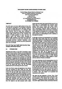
N W

RELATED WORK

Regarding the field of intelligent transportation systems (ITS), there are vast number of researches and work being developed under the umbrella of traffic lights control using wireless sensor networks. In [7], an algorithm for traffic signals using sensors was designed and implemented. This algorithm was implemented using MATLAB, whereas hardware simulation of the sensor nodes were by LabVIEW. However, it did not show the vehicles behaviour under the mentioned work (e.g., average waiting and travel time of vehicles), nor shows the sensors communications-related data (e.g., number of transmitted frames, frames collisions, MAC protocol used, etc.). In [8], the authors used a wireless sensor networks of two models (one and two sensor nodes) and compared the performance between those models according to the average trip waiting time. The authors did not provide telecommunications aspects of the sensor nodes. In [9], an alerting system for red light crossing scenarios in addition to the traffic light control algorithm presented for different models, has been implemented to alert the drivers in other sides to reduce the chance of accidents due to red light crossing violations using sensors according to lane occupancies. It had not used specific type of sensors, instead, mentions types that can be used (ultrasonic vehicle detector or cameras) to calculate the queue (lane) length. In [10], the authors addressed the intersection throughput alongside with average vehicular waiting time by proposing an adaptive traffic light control algorithm for isolated intersection running in multiple steps. Then, they compared the proposed algorithm against fixed-time and traffic-actuated counterparts. Additionally, the authors did not address the communications aspects nor specify the type of sensors used to detect vehicles IDs and vehicles types. In [11], a sensor network architecture that does not depend on a centralized coordinator and separate it logically into four hierarchical levels was proposed. These levels are final computations/decision (layer 4), intermediate computations (layer 3), departures detection (layer 2), and arrivals detection (layer 1). It used conflict matrix to specify the desired behaviour of each intersection. However, the cost of adding a leader election (when a sensor’s battery drops below a threshold) and self-organizing protocols were not explained enough, and no information about their batteries consumption rate or sensors telecommunications properties provided. The authors of [12] extended their previous work of [11] with a special focus on communications and studying its reaction to losses and delays induced by the use of wireless communication. Although [11] provided a state-of-the-art work and proved the efficiency and ease of implementation of their algorithm of [13] , their work, and all previous [7, 8, 9, 10, 11], have not showed energy consumption for sensor nodes batteries under their proposed sensor network architecture and/or adaptive traffic signals algorithms.

E

1 1

S

5

6: W arrival sensor

6

Sensors Level 1 Level 2

1: N arrival sensors

5: E arrival sensor

3 3

3: S arrival sensors

Fig. 1: Our hierarchical model.

3.1

Network Architecture

Our proposed wireless sensor network architecture is shown in Fig. 1. It has no centralized station that coordinates the traffic controllers’ behaviour, but rather, each traffic signal controls the intersection locally without the help of external entity. It consists of two levels of hierarchies only. Level 1 consists of one sensor node per lane for detecting the presence of vehicle arrivals. Each sensor node is encased in a 5” diameter glued into the pavement of the lane. Vehicles are detected due to the change in the earth’s magnetic field caused by the arrival of the vehicles above the sensor node [14]. Level 2 are the traffic signals that retrieve the sensor nodes information and acts upon them. Level 2 are the traffic signals themselves. It means that, traffic signals are sensor nodes too, but are externally powered, in contrast with level 1 sensors, which use batteries (internally powered).

3.2

Traffic-actuated signals

Traffic-actuated control of isolated intersections attempts to adjust green time continuously, and, in some cases, the sequence of phasing. These adjustments occur in accordance with real-time measures of traffic demand obtained from vehicle detectors (sensor nodes in this work) placed on one or more of the approaches to the intersection. The full range of actuated control capabilities depends on the type of equipment employed and the operational requirements [1]. Fig. 2 shows its phasing diagrams [1]. This general and simple detection algorithm acts as the main algorithm that our architecture for this work has been applied to it. Fig. 3 is the corresponding flowchart of it. As can be seen in the flowchart, it is a continuous operation, since traffic lights should control intersections all the time long.

TRAFFIC LIGHTS CONTROL ARCHITECTURE

3.2.1 Actuated phasing parameters. Each phase can either be served or skipped. The decision to skip a phase occurs when there is no vehicle on the detector when the previous phase turns yellow. If a phase is served, it is served for a minimum period called the minimum green or initial. After the initial, the phase will rest in green until a car passes over a detector on a competing phase. At that point, the phase can be terminated by one of two processes (in our work) [2]:

The following section illustrates the proposed single sensor per lane architecture and description about the inner layers of it; followed by the traffic control algorithm that had been executed in order to measure the effectiveness of our architecture.

Gap-out. As soon as a competing phase has been called, the phase showing green will start a timer, called the extension timer, which counts down from the extension value to zero.

3.

2

International Journal of Computer Applications (0975 8887) Volume 104 - No. 12, October 2014

Fig. 6: Induction loops placements.

Fig. 2: Traffic-actuated phase timing diagram.

Beginning of phase due to actuation or recall

Extensible green

4.1

Yes

Max Green?

Sensed?

Yes

Gap?

Yes

Yellow Red

Yes

Sensed?

Fig. 3: Flowchart of Fig. 2 (empty edges represent No output).

Max-out. If traffic is heavy, a sufficient gap to gap-out may not occur in a reasonable period. Thus the actuated controller provides a maximum time to prevent excessive cycle lengths.

4.

so that information from SUMO been reflected back to OMNeT++, on the same working area but with other type of simulation. The following sections gives basic definitions of both SUMO and OMNeT++ and the area under study that have been simulated by them, followed by the parameters that is been used for traffic signals (fixed and actuated) in SUMO and the parameters of the channel and wireless sensor nodes used in OMNeT++. Finally, the work results are shown at the end of this section.

EXPERIMENTAL SETUP AND RESULTS

This study combines the results of two simulators, SUMO (described below) that is used for vehicular simulation and OMNeT++, which is a network simulator. Those two simulators were connected

SUMO

SUMO, Simulation of Urban MOblity, is an open source, highly portable, microscopic and continuous road traffic simulator designed to handle large road networks [5]. Fig. 4 shows the map of the city that is been used under study. In order to use those maps with SUMO, the street/road type map should be converted to SUMO map network file. The equivalent SUMO map of the city is shown in Fig. 5. 4.1.1 Induction loops. Traffic-actuated signals vary their green time based on demand at the intersection as measured on detectors installed on the approach. These detectors vary in technology, but the most common is the inductive loop detector. Induction loops are provided in SUMO, so that when a particular vehicle is passed above the induction loop, this information can be obtained by means of TraCI, the short term for ”Traffic Control Interface”; giving the access to a running road traffic simulation, it allows to retrieve values of simulated objects and to manipulate their behaviour ”on-line” [15]. Interfacing with TraCI can be done with Python or Java programming languages1 . Induction loops (sensor nodes) placements. Induction loops (sensor nodes) placements depends heavily on the traffic data for a given intersection, the placements of induction loops inside SUMO were 25 meters from the edge of the lane, so that the vehicle has a chance of green time before the gap-out is been reached ( [16] recommends a distance of 61 to 76.2 m in urban areas, but it also says “distance depends on cycle length, split, and offset”). Fig. 6 shows the placement of induction loops (yellow rectangles) for one of the intersections (intersection 3) in the city being simulated. 1 This

work uses Python interface with TraCI.

3

International Journal of Computer Applications (0975 8887) Volume 104 - No. 12, October 2014

(a) Sattellite map

(b) Street/road map

Fig. 4: The city under simulation (Adhamiyah, Baghdad).

Fig. 5: SUMO network map for the city of Adhamiyah.

OMNeT++ is an extensible, modular, component-based C++ simulation library and framework, primarily for building network simulators [6]. MiXiM is an OMNeT++ modelling framework created for mobile and fixed wireless networks (wireless sensor networks, body area networks, ad-hoc networks, vehicular networks, etc.) [17]. It offers detailed models of radio wave propagation, interference estimation, radio transceiver power consumption and wireless MAC protocols (e.g. Zigbee). This paper uses MiXiM framework for modelling the IEEE 802.15.4 wireless sensor nodes in OMNeT++. Wireless sensor nodes retrieves the sensing information from the induction loops of SUMO, by means of TCP communication between the two simulators.

:X

OMNeT++

φ x

SUMO side

Connecting SUMO and OMNeT++ In order to to transfer the presence of vehicles from induction loops in SUMO to OMNeT++ sensor nodes, i.e., to connect the two simulators, inter-process communication by means of sockets has been established between them. SUMO sockets were been programmed in Python and OMNeT++ sockets were in C++. See Fig. 7.

4.3

Senso r Nod e ID

4.2

x

OMNeT++ side

Φ: Induction Loop ID: X (Inter-process communication)

Fig. 7: Overview of simulators cooperation.

Traffic signals parameters

Table 1 shows the parameters of both fixed-time and trafficactuated signals used in SUMO. Fixed-time signal parameters

were default in SUMO, and traffic-actuated signals had been programmed and fine-tuned to get better results.

4

International Journal of Computer Applications (0975 8887) Volume 104 - No. 12, October 2014 Table 4. : Channel parameters

Table 1. : Traffic signals parameters Fixed-time signals Parameter name

Value (seconds)

Green time Yellow Change Interval Red time Leading left green time Leading left yellow interval Cycle length

31 9 56 46 9 112

Parameter name

Value

Maximum sending power used for this network Minimum signal attenuation threshold Minimum path loss coefficient

2 mW −100 dBm 2.5

traffic signals does not transmit any information or require specific type of data to be simulated in OMNeT++.

Traffic-actuated signals Parameter name

Value (seconds)

Minimum green Gap-out Max-out Yellow Change Interval Leading left green time Leading left yellow interval

5 5 20 2 9 2

Table 2. : Sensor nodes parameters Parameter name

Value

Sensitivity Maximum transmission power Initial radio state Use thermal noise Carrier frequency Modulation type MAC Protocol

−100 dBm 1.1 mW TX true 2.4 MHz MSK CSMA

Table 3. : Battery specifications Parameter name Capacity Voltage

4.4

Value 6600 mAh 3.3 V

Sensor nodes parameters

MiXiM model framework in OMNeT++ implements the IEEE 802.15.4 narrowband protocol, which is being used as the protocol for the wireless sensor nodes that sense the vehicles from SUMO, and then send the data to its traffic signal in order to perform its intended operation. Table 2 contains the specifications of those sensor nodes. Since wireless sensors nodes have no external power, i.e., they use batteries, table 3 contains the battery specifications for the wireless sensor nodes. Other information that should be mentioned are the channel parameters, which are listed in table 4. Traffic-actuated signals in OMNeT++ were simulated with parameters just like the sensor nodes, but without batteries, that is, they’re externally powered (due to their conditions of consuming and processing much more data than with sensor nodes, and due to the fact the LED traffic lights cannot be powered by batteries for a very long time, e.g., years). For setting the traffic signals phases in SUMO, the Python interface of TraCI were used, instead of transferring the decisions from OMNeT++ C++ code to SUMO Python, since

4.5

SUMO results

One of the important parameters that is to be enhanced is the (average) vehicular waiting time. Fig. 8 shows the average vehicular waiting and travel times of both fixed-time and traffic-actuated signals, where V is the average velocity. The horizontal axes contains the number of vehicles while the vertical contains the delay in seconds. There are six samples within each scenarios (six for fixed-time and the same for traffic-actuated). In both scenarios, the same city (has three intersections) and the number of vehicles and their parameters (i.e., acceleration, length, maximum speed, driver’s imperfection, etc...) were all the same prior to the operation of traffic signals, in order to make the comparison with the same attributes. As can be seen, traffic-actuated signals have better results than its counterpart. The total average waiting time for fixed-time signal is 495 seconds, while the other has 210 seconds, which shows that traffic-actuated signals have enhancements by a factor of about 42%. Induction loops (sensor nodes). Induction loops (sensor nodes in OMNeT++) were the primary source of information in our simulation results. Each induction loop in SUMO saves information to a file by freq attribute, which is the aggregation period the values the detector collects shall be summed up. For our simulation study, which has three intersections, induction loops from 0 − 8 were assigned for the first intersection, 9 − 20 for the second intersection and 21 − 28 for the third intersection. Fig. 9, 10 and 11 show the average lengths, occupancies and speeds, respectively, of the vehicles, retrieved from induction loops information for the second sample of the traffic-actuated signals (i.e., with the 1989 number of vehicles). As can be seen from the figures, there were a total of 29 (from 0 − 28 induction loops planted in the city around the intersections. The horizontal axes contains the identification numbers (ids) of induction loops (sensors). It can be noticed that most of the sensed vehicles have a length of 5 meters, which is the default vehicle length in SUMO. Our work has added different lengths in order to have more ranges of lengths in our simulation. The vertical axes for the values of the occupancies is a percentage (0 − 100%) of the time a vehicle was at the detector.

4.6

OMNeT++ results

After the wireless sensor nodes been defined in OMNeT++ and been synchronized with induction loops of SUMO, another different types of data were been given. Fig. 12 shows the number of sensed vehicles for each wireless sensor node from the same second sample of the simulation (i.e., with the 1989 number of vehicles). As can be seen, sensor node with id of 11 has the highest detection of vehicles (909).

5

International Journal of Computer Applications (0975 8887) Volume 104 - No. 12, October 2014

Fixed-time signals Average waiting time Average travel time

1400

Traffic-actuated signals 1400 1200

1000

1000

seconds

1200

800

800

600

600

400

400

200

200

0

957

1989 V=6

V=10

2905

3966 V=7

V=10

vehicles

4861 V=8

5849 V=8

0

957

V=12

1989

2905

V=10

3966

V=12

V=10

4861

V=11

5849

V=11

Fig. 8: Average waiting and vehicular times of traffic signals (V is the average velocity). 8

30

7

25

6 20

meters

m/s

5 4 3

15 10

2

5

1 00

5

15

10

nodes ids

20

00

25

5

10

15

nodes ids

20

25

Fig. 11: Average speeds of vehicles. Fig. 9: Average lengths of vehicles. 30 800

#cars sensed

25

%

20 15 10

600

400

200

5 00

00

5

10

15

nodes ids

20

25

5

10

15

nodes ids

20

25

Fig. 12: Number of sensed cars per sensor node.

Fig. 10: Average occupancies of vehicles.

Fig. 13, 14, 13 and 16 show the number of transmitted frames with and without interference, the number of received frames (since the

6

International Journal of Computer Applications (0975 8887) Volume 104 - No. 12, October 2014

50

#dropped frames

#transmitted frames

800

600

400

200

40 30 20 10

00

5

10

15

nodes ids

20

00

25

Fig. 13: Number of transmitted frames per sensor node.

5

10

15

nodes ids

20

25

Fig. 16: Number of dropped frames.

1.4

800

1.0

#backoffs

#frames with interference

1000

1.2

0.8 0.6

600 400

0.4 200

0.2 0.0 0

5

10

15

nodes ids

20

00

25

10

15

nodes ids

20

25

Fig. 17: Number of backoffs.

Fig. 14: Number of frames with interference. 2.0

3000 2500

1.5

seconds

#received frames

5

2000 1500 1000

1.0

0.5

500 00

5

10

15

nodes ids

20

25

Fig. 15: Number of received frames per sensor node.

CSMA MAC protocol is used, that is, it tries to detect the presence of a carrier wave from another node before attempting to transmit), and the number of dropped frames, respectively, for each sensor node. Since sensor node 11 has the highest number of sensed vehicles, it is not surprising that it is also the highest node for transmitting frames.

0.0 0

5

10

15

nodes ids

20

25

Fig. 18: Backoffs durations.

Because sensor nodes from 9−20 belong to the second intersection, Fig 15 shows those nodes have the highest network traffic among all other sensor nodes. Since the MAC protocol used here is CSMA, when the medium is busy, the node performs a backoff operation, that is, it waits for a certain amount of time before attempting to transmit again. Fig. 17 and 18 shows the relative backoff information of the sensor nodes.

7

International Journal of Computer Applications (0975 8887) Volume 104 - No. 12, October 2014

5.

CONCLUSION

Because of the diverse applications of sensor networks in every day life, they’ve been employed in our work for traffic controls by reporting the traffic movements. We used them as means of enhancing traffic flow by reducing average vehicular waiting time, which proves to be more efficient than with fixed-time signals. We proposed and simulate a simple, cheap but efficient sensor network architecture composed of only a single sensor node per lane. In order to measure the effectiveness of our architecture, we executed a simple actuated (adaptive) traffic algorithm so that to lengthen the duration of sensors’ life (instead of a complex one), which can be beneficial for countries that want to apply economic solutions to traffic control. As a future work, we would like to simulate coordinated traffic signals, as traffic signals would cooperate among them to further enhance the traffic flow.

6.

REFERENCES

[1] “Trafficware resources - reference documents, signal timing.” http://www.trafficware.com/resources. Accessed: 2014-05-26. [2] M. Kutz, Handbook of Transportation McGraw-Hill handbooks, Mcgraw-hill, 2003.

Engineering.

[3] “Directive 2010/40/eu of the european parliament and of the council of 7 july 2010 on the framework for the deployment of intelligent transport systems in the field of road transport and for interfaces with other modes of transport.” http: //eur-lex.europa.eu/LexUriServ/LexUriServ.do? uri=OJ:L:2010:207:0001:0013:EN:PDF. Accessed: 2014-06-28. [4] W. Dargie and C. Poellabauer, Fundamentals of wireless sensor networks: theory and practice. John Wiley & Sons, 2010.

[11] S. Faye, C. Chaudet, and I. Demeure, “A distributed algorithm for adaptive traffic lights control,” in Intelligent Transportation Systems (ITSC), 2012 15th International IEEE Conference on, pp. 1572–1577, IEEE, 2012. [12] S. Faye, C. Chaudet, and I. Demeure, “Influence of radio communications on multiple intersection control by a wireless sensor network,” in ITS Telecommunications (ITST), 2013 13th International Conference on, pp. 307–312, IEEE, 2013. [13] S. Faye, C. Chaudet, and I. Demeure, “A distributed algorithm for multiple intersections adaptive traffic lights control using a wireless sensor networks,” in Proceedings of the first workshop on Urban networking, pp. 13–18, ACM, 2012. [14] S. Y. Cheung, S. C. Ergen, and P. Varaiya, “Traffic surveillance with wireless magnetic sensors,” in Proceedings of the 12th ITS world congress, pp. 1–13, 2005. [15] A. Wegener, M. Piorkowski, M. Raya, H. Hellbrck, S. Fischer, and J.-P. Hubaux, “TraCI: An Interface for Coupling Road Traffic and Network Simulators,” in 11th Communications and Networking Simulation Symposium (CNS), 2008. [16] R. L. Gordon, W. Tighe, and I. Siemens, Traffic control systems handbook. US Department of Transportation, Federal Highway Administration, Office of Operations, 2005. http: //ops.fhwa.dot.gov/publications/fhwahop06006/ Accessed: 2014-06-09. [17] A. K¨opke, M. Swigulski, K. Wessel, D. Willkomm, P. T. K. Haneveld, T. E. V. Parker, O. W. Visser, H. S. Lichte, and S. Valentin, “Simulating wireless and mobile networks in omnet++ the mixim vision,” in Proceedings of the 1st International Conference on Simulation Tools and Techniques for Communications, Networks and Systems & Workshops, Simutools ’08, (ICST, Brussels, Belgium, Belgium), pp. 71:1–71:8, ICST (Institute for Computer Sciences, Social-Informatics and Telecommunications Engineering), 2008.

[5] D. Krajzewicz, J. Erdmann, M. Behrisch, and L. Bieker, “Recent development and applications of SUMO - Simulation of Urban MObility,” International Journal On Advances in Systems and Measurements, vol. 5, pp. 128–138, December 2012. [6] A. Varga and R. Hornig, “An overview of the omnet++ simulation environment,” in Simutools ’08: Proceedings of the 1st international conference on Simulation tools and techniques for communications, networks and systems & workshops, (ICST, Brussels, Belgium, Belgium), pp. 1–10, ICST (Institute for Computer Sciences, Social-Informatics and Telecommunications Engineering), 2008. [7] A. Albagul, M. Hrairi, M. Hidayathullah, et al., “Design and development of sensor based traffic light system,” American Journal of Applied Sciences, vol. 3, no. 3, p. 1745, 2006. [8] M. Tubaishat, Q. Qi, Y. Shang, and H. Shi, “Wireless sensorbased traffic light control,” in Consumer Communications and Networking Conference, 2008. CCNC 2008. 5th IEEE, pp. 702–706, IEEE, 2008. [9] F. A. Al-Nasser and H. Rowaihy, “Simulation of dynamic traffic control system based on wireless sensor network,” in Computers & Informatics (ISCI), 2011 IEEE Symposium on, pp. 40–45, IEEE, 2011. [10] B. Zhou, J. Cao, X. Zeng, and H. Wu, “Adaptive traffic light control in wireless sensor network-based intelligent transportation system,” in Vehicular Technology Conference Fall (VTC 2010-Fall), 2010 IEEE 72nd, pp. 1–5, IEEE, 2010.

8