Simulation and Test-Case Generation for PVS ... - CiteSeerX

International Journal on Advances in Software, vol 4 no 3 & 4, year 2011, http://www.iariajournals.org/software/

327

Simulation and Test-Case Generation for PVS Specifications of Control Logics Cinzia Bernardeschi, Luca Cassano, Andrea Domenici Department of Information Engineering University of Pisa, Italy {c.bernardeschi, l.cassano, a.domenici}@ing.unipi.it

Abstract—We describe a framework for the simulation of control logics specified in the higher-order logic of the Prototype Verification System. The framework offers a library of predefined modules, a method for the composition of more complex modules, and an event-driven simulation engine. A developer defines a system architecture by composing its model out of library modules, possibly introducing new module definitions, and simulates the behaviour of the system model by providing its input waveforms, which are given as functions from time to logic levels. The generation of simulation scenarios (test cases) can be automated by using parametric waveforms that can be instantiated through universal and existential quantifiers. We demonstrate the simulation capabilities of our framework on two simple case studies from a nuclear power plant application. The main feature of this approach is that our formal specifications are executable. Moreover, once the simulation experiments give developers sufficient confidence in the correctness of the specification, the logic models can serve as the basis for its formal verification. Keywords-PVS; simulation; validation; test-case generation; control logics.

I. I NTRODUCTION AND MOTIVATION Control systems combine real-time requirements and nontrivial control tasks whose failure may compromise safety. Subtle design faults, difficult to avoid and tolerate, and the possibility of failures caused by the occurrence of non-obvious combinations of events, make such systems hard to certify with respect to safety requirements. The use of formal methods is increasingly being required by international standards and guidelines for the development of safety critical digital control systems. Formal methods are in fact recognised as a fault avoidance technique that can increase dependability by removing errors at the requirements, specification and design stages of development. In this paper, we present a methodology (introduced in [1]) for the simulation of control logics, formally specified in the higher-order logic of the Prototype Verification System (PVS) [2], a specification and verification system that combines an expressive specification language with an interactive theorem prover. Thus, the same model can be used both for simulation and formal verification of system properties. Formal methods are highly recommended by such standards as the EN 50128:2001 European Standard [3] in the requirements specification and in the design and the validation of

Paolo Masci School of Electronic Engineering and Computer Science Queen Mary University of London, UK [email protected]

railway control and protection systems, and the IAEA NSG-1.1 Standard [4] in digitalised instrumentation and control systems in nuclear power plants. On the other hand, verification and validation (V&V) of embedded systems relies heavily, and often exclusively, on simulation and testing. In particular, simulation is often the only V&V tool in the development of ASIC- and FPGA-based hardware. A typical development process for such systems involves creating a block-diagram model through a CAD tool that generates a model of the hardware at successive levels of detail, and each of these intermediate models is simulated. Alternatively, the initial model may be expressed in a hardware description language such as Verilog [5] or VHDL [6]. A rigorous development process would benefit from the combined application of formal verification, simulation, and testing. In particular, simulation would be a means to validate specifications against requirements. However, verification tools (such as theorem provers and model checkers) and simulation tools use different languages, and few designers are versed in the use of both kinds of tools. The work presented in this paper is focused on the validation of high level specifications of control logics, relying on executable formal specifications. We note that executable specifications are more commonly based on process algebras or state machine formalisms that are more amenable to computer execution than logic-based formalisms, but they suffer the problem of state explosion [7]. It is assumed that the development process of a control system starts from a specification expressed as function block diagrams. This specification can be translated into a highorder logic theory that guides the execution of a simulator. When the simulation results make developers confident that their specifications express the intended system behaviour, a more detailed and formal analysis of its properties may be done by theorem proving. In function block diagrams, each block represents some operation on digital or analog signals. Such operations include, for example, Boolean functions, comparison, voting, integration and differentiation. Functional blocks may be implemented in many ways: a single functional block may correspond to one or more hardware modules, a group of blocks may be implemented in a single hardware module, and a block or group may be implemented in software executed

2011, © Copyright by authors, Published under agreement with IARIA - www.iaria.org


328 by some programmable device. This work addresses systems where only digital (i.e., discrete-valued) signals are present. We have developed a library of purely logic specifications for typical control system components, a methodology to combine them into more complex systems, and a simulation engine capable of animating the formal specifications with the PVS ground evaluator. The library comprises definitions for basic concepts, such as time, signals, and events. The simulation framework also enables test cases (input data to the simulations) to be automatically generated by using parametric waveforms that can be instantiated through universal and existential quantifiers. The paper is organised as follows. Section II reports related work on formal verification of digital control systems. We introduce the PVS system in Section III, then we describe the theories for the logical specification of signals and control components (Section IV) and the theory defining the simulator including a theory for the events associated to signals (Section V). In Section VI, we describe two simple case studies from the field of control logics for nuclear power plants (NPPs), and, finally, the conclusion is found in Section VII. II. R ELATED W ORK The last few years have seen a continuous increase in usage of digital components in safety critical control systems. Digital control systems are flexible and enable sophisticated control schemas to be realized. However, these systems are complex and call for advanced tools and techniques to ensure compliance with safety requirements. A few examples in the literature point out to the difficulties in anticipating all risk situations and to the fact that apparently harmless events (such as small unforeseen changes in a sequence of operations) may lead to catastrophic consequences. These reasons motivate the introduction of formal methods in the development process of control systems as early as their first phases (as acknowledged by international standards). Such methods afford a precise representation of control schemas and make it possible to reason on control systems properties in a rigorous manner. The application of these methods, however, must deal with the problem of complexity of the systems to be analysed and is therefore an advanced research topic with interesting theoretical implications and relevant practical advantages. In many research works, digital control system specifications are analyzed with logical-mathematical methods. Two lines of research emerge from these works, addressing methods based on model checking [8] and theorem proving [9], respectively. Model checking relies on generating a state model of system behavior. Properties expressed in temporal logic are automatically verified by model-checking algorithms. Theorem proving relies on a logic language and a collection of inference rules specific of each language. Verification is done by proofs assisted by a theorem proving tool that can apply inference rules in an entirely or partially automatic manner. Several works have explored the use of model checkers and theorem provers in the field of instrumentation and control. For instance, Krämer et al. [10] used the Isabelle/HOL

theorem prover for modelling and verifying programs for programmable logic controllers. They demonstrated the utility of using formal methods on such systems, and in particular they argued that the sheer exercise of formalising system descriptions given with graphical languages, such as function block diagrams, is able to point out incomplete information about functionalities, ambiguities, contradictions and design flaws. Wan et al. [11] used the Coq theorem prover for modelling and verifying programs for programmable logic controllers with timers. They addressed the problem of reasoning on specifications that involve timers, and they propose a set of axioms suitable to ease the modelling of timers at different levels of abstraction. Jee et al. [12] translated function block diagrams into semantically equivalent Verilog programs that can be checked with the SMV model checker, and they implemented also a visualisation tool for animating the specifications. Various works, like Vyatkin and Hanisch [13], and Missal et al. [14], translated function block diagrams into Signal Net Systems, a generalisation of Petri Nets, and then used ad hoc analysis tools for analysing properties of interest on the Signal Net System specification, such as reachability of dangerous states and validation of arbitrary input/output specifications. VHDL and Verilog are commonly used for logical circuits design. Their key advantage is that they allow the behaviour of a system to be modeled and simulated before synthesis tools translate the design into real hardware. The problem of formal verification of VHDL designs is dealt with in [15] where the behaviour of a VHDL design is specified with temporal logic formulas and a model checker is applied for the verification of the design. In [16], a language to design circuits and prove properties in the Nqthm theorem prover [17] is shown. The language can be translated to a subset of VHDL. Jain et al. [18] verified circuits described in Verilog with a model checking and predicate abstraction technique, and developed a model checking tool, VCEGAR, suitable to verify safety requirements of control system specified in Verilog [19]. The model checking analysis of complex control systems suffers of the state-space explosion problem, thus requiring abstraction techniques where verification is performed on a set of abstract states. Theorem provers are fundamental in this application field, even if this kind of tools requires specific competence of the control designer and verification is semiautomatic. In our work, on the other hand, we have investigated the possibility of integrating an event-based simulation environment into a theorem proving system: simulations give designers an intuitive and effective way for investigating the behaviour of a system through test cases; theorem proving enables analysts to explore all possible behaviours of the system, which is essential in safety critical domains for detecting design errors in advance. PVS is currently one of the most popular and powerful theorem provers, that has been used for formal reasoning in several application domains [20]. In particular, it has been



329 used in various works to specify and verify hardware systems, e.g., in [21][22][23]. Other application fields include fault tolerant systems [24], wireless sensor network protocols [25], and distributed cognition systems [26]. With our approach, the formal specifications are executable and they can be simulated with the ground evaluator of PVS. This way, once the simulation experiments give developers sufficient confidence in the correctness of the specification, the same PVS models can serve as the basis for the formal verification of properties in the theorem prover of PVS. It is known that a large share of defects in computing systems stem from errors in the formulation of specifications [27]. III. PVS AND PVS IO The distinguishing characteristics of PVS [2] are its expressive specification language and its powerful theorem prover. The PVS specification language builds on classical typed higher-order logic with the usual base types, bool, nat, integer, real, among others, and the function type constructor (e.g., type [A -> B] is the set of functions from set A to set B). Predicates are functions with range type bool. The type system of PVS also includes record types, dependent types, and abstract data types. PVS specifications are packaged as theories that can be parametric in types and constants. A collection of builtin (prelude) theories and loadable libraries provide standard specifications and proved facts for a large number of theories. A theory can use the definitions and theorems of another theory by importing it. For instance, consider the following theory execution: execution: THEORY BEGIN State: TYPE tf : VAR [State -> State] execute(n_steps: nat)(tf): RECURSIVE [State -> State] = LAMBDA (s: State): IF n_steps = 0 THEN s ELSE LET s_prime = tf(s) IN execute(n_steps - 1)(tf)(s_prime) ENDIF MEASURE n END execution

The theory defines a State and a (higher-order) function execute that recursively applies n_steps of a statetransition function tf, that is provided as a parameter. As all functions in PVS must be total, the termination of the recursion has to be demonstrated; the MEASURE part provides the information to the typechecker and prover to ensure this. Thus, the execution theory provides a generic mechanism to describe the execution of a system, that can subsequently be used for simulation. The PVS environment has an automated theorem prover that provides a collection of powerful primitive inference procedures that are applied interactively under user guidance within a sequent calculus framework. The primitive inferences include propositional and quantifier rules, induction, rewriting,

simplification using decision procedures for equality and linear arithmetic, data and predicate abstraction [28]. Although PVS offers a very expressive specification language, a large subset of the language is actually executable: all ground expressions of ground type are executable; the only fragments of the language that are not executable are uninterpreted functions, quantification over infinite domains, free variables, and equalities between higher-order terms. However, the evaluation is nonstrict, and expressions may be executed even if they contain unexecutable subexpressions. PVS includes a ground evaluator [29] that can be used to evaluate, test, and animate PVS specifications by executing them on concrete data. The core of the ground evaluator is a translator that compiles executable PVS expressions into Common Lisp code. The translation is performed lazily, i.e., the translation of an expression happens only when its value is actually required. The ground evaluator also consists of an evaluation environment, which is an interactive read-eval-print loop that allows the user to input expressions, and returns the result of their evaluation. The techniques used in the ground evaluator to associate Lisp programs with PVS functions are also available to the PVS user, who can provide pieces of Lisp code (called semantic attachments) and attach them to PVS symbols. This mechanism is useful to allow expressions that involve unexecutable constructs, such as uninterpreted functions, to be handled by the evaluator, by associating them with a suitable implementation. Using this mechanism, the PVSio package [30] extends the ground evaluator with a predefined library of imperative programming language features such as side effects, unbounded loops, and input/output operations, and also provides a highlevel interface for writing user-defined semantic attachments. Thus, PVS specifications can be conveniently animated within the read-eval-print-loop of the ground evaluator. In our framework, we exploit the expressiveness of the PVS specification language for enabling a natural mapping between higher order logic specifications and systems models described as function block diagrams. We employ the mechanisms provided by PVSio for implementing a customisable simulation environment suitable to animate the model of the system expressed in higher order logic. IV. M ODELLING C ONTROL L OGICS In this section, we describe the PVS theories developed to formally model control logics. We start with the PVS theories that model time, logic levels, signals, and basic operations on signals. Then, we introduce samples of the library for the basic digital modules of a system, such as logic gates and timers. Finally, we show how to build complex components out of basic elements. The developed theories are executable: definitions always use interpreted types and quantification is always performed over bounded types. In the following sections, only the time_th theory will be shown in a syntactically complete form; only some relevant fragments



330 of PVS code will be shown in the rest of the paper for the other theories. A. Time Time is modelled as a variable ranging over the continuous domain of real numbers. Theory time_th (shown below) contains the type definition of time (modelled as ranging over the continuous domain of real numbers) and time interval. In the theory, time represents the relative time with respect to an initial time. The initial time is the zero reference point: negative time values represent time instants preceding the initial time, while positive time values represent time instants following the initial time. Type interval models time intervals with a non-negative real number (instantaneous time intervals have duration zero). time_th: THEORY BEGIN time: TYPE = real interval: TYPE = {t: time | t >= 0} END time_th

B. Logic Levels The logic levels of hardware circuits correspond, in the real world, to voltage or current levels. Besides the classical zero and one values, additional levels are needed to model unknown values and high impedance. Unknown values are useful to model the logic level when the digital circuit is powered up, while high impedance is useful to represent open circuits or mis-wiring situations (e.g., the designer forgets to wire a port of the digital circuit). Theory logic_levels_th provides the definitions of the logic levels and of the logical operators over the four-valued logic. In the theory, logic levels are modelled with natural numbers (each level is associated with a unique number), and each level is associated with a mnemonic name and a recogniser predicate (denoted by the mnemonic name followed by a question mark symbol). In the following fragment, we show the definitions of types and constants, and the definition of the basic logical operator lAND over the four-valued logic. Other definitions are in Appendix A. logic_levels_th: THEORY BEGIN %-- logic level (type definition) logic_level: TYPE = below(4) %-- names of logic levels zero: logic_level = 0 one: logic_level = 1 Z: logic_level = 2 %-- high impedance U: logic_level = 3 %-- unknown %-- logical AND in a four-valued logic lAND(v1, v2: logic_level): logic_level = IF one?(v1) AND one?(v2) THEN one ELSIF zero?(v1) OR zero?(v2) THEN zero ELSE U ENDIF % ... END logic_levels_th

C. Signals A signal describes the variation of a logic level over time, and we represent signals as functions from the domain of time to logic levels. Signal transitions are specified pointwise, by comparing the logical level of the signals at two closely spaced time points. The spacing between time points corresponds to the time resolution of the digital circuit, i.e., the minimum amount of time required by the components in the circuit for detecting two observable variations of a signal. This allows us to simplify the definition of signals transitions, and also to define executable functions for detecting signals transitions over the continuous time domain. Note that the generality of properties proved on specifications involving the concept of time resolution does not affected the generality of the proof, because the actual value of the time resolution can be left unspecified (i.e., any value is possible) when doing the proof. Theory signals_th contains, besides the definition of signal, the symbolic constant for time resolution, tres, which models the minimum time between two observable variations of a signal, and the definitions of utility functions to shift a signal in time (time_shift) and to build periodic signals (periodic). Basic signals provided in the theory are: constval, a constant logical level; step, a signal that goes from zero to one at time τ ; pulse, a signal that is one only in the time interval [τ, τ + d), where d is the interval size. Some useful predicates on signals are defined, such as rising_edge?, used to detect if a signal s has a rising edge at time tau. Logical operations on signals are defined (sOR, sAND, sNOT), that apply the operator to the values of signals at each given time. Sample definitions of this theory follow. More definitions are in Appendix A. signals_th: THEORY BEGIN IMPORTING time_th, logic_levels_th %-- signal (type definition) signal: TYPE = [time -> logic_level] %-- symbolic constant of the minimum time % between two observable variations in a signal tres: posreal %-- definition of basic waveforms step(tau: time): signal = LAMBDA (t: time): IF t >= tau THEN one ELSE zero ENDIF % ... %-- time shift of the signal time_shift(s: signal, offset: time): signal = LAMBDA (t: time): s(t - offset) %-- logical operators in a four-valued logic sAND(s1, s2: signal): signal = LAMBDA (t: time): IF one?(s1(t)) AND one?(s2(t)) THEN one ELSIF zero?(s1(t)) OR zero?(s2(t)) THEN zero ELSE U ENDIF % ... END signals_th



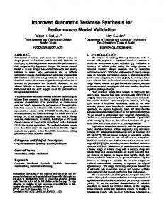
331

r

q

r x 00 x01

y0 q

G0

SR s

q’ s x10 x11

y1 q’

G1

(a)

(b) Fig. 1.

An SR flip-flop.

D. Digital Modules In our framework, a control logic is a composite digital module, obtained by connecting basic digital modules. Digital modules are characterised by a set of ports, a state, and a transition function. Ports are abstractions of the terminals of physical devices. Each port is identified by its category (one of input, output, internal) and its port number within the category. Basic modules have only input and output ports, whereas composite modules also have internal ports. In a composite module, the input and output ports are its externally visible terminals, and its internal ports are the ports of the (basic) component modules that are not externally visible. For example, a NOR gate is modelled as a module with two input ports, one output port, and no internal ports. Another example is an SR flip-flop, which can be modelled either as a basic module (Figure 1(a)) with two input ports, two output ports and no internal ports, or as a composite module built from two NOR gates. In this case, the resulting system is shown in Figure 1(b), where ports x00 of gate G0 and x11 of gate G1 are input ports, ports y0 of G0 and y1 of G1 are output ports, and ports x01 and x10 are internal ports. The state of a module is defined as the set of signals (i.e., functions of time modelling waveforms) applied to, or generated by, the module at a given time. Defining the state as a set of time functions instead of instantaneous values makes it possible to define the behaviour of some modules in terms of properties of such functions, thus allowing for better expressiveness. As an example, we may consider the specification of a timer, whose output depends on the shape (namely, the presence of a rising edge) of its input signal, along with the current value of the output: timerM(d: posreal): basic_digital_module(1, 1) = LAMBDA (t: time): LAMBDA (s: state(1, 1)): IF rising_edge?(port0(input(s)), t) AND zero?(port0(output(s)), t) THEN s WITH [output := ports(pulse(t + delay, d))] ELSE s ENDIF

With this approach, a state transition occurs when a signal on a port is replaced by a different one. For example, let us consider the timer defined above, timerM. Let us suppose that the initial signals on the output port of the timer is a constant logical zero (constval(zero)) and that the input signal is a step, with rising edge at t = t∗ (step(t_star)). As long as t < t∗ , the output signal remains a constant logical zero, because the condition expressed in timerM is false. When t = t∗ , the condition in timerM becomes true, and the state changes: the constant logical zero signal on the output port is replaced with a pulse signal of duration d starting after a propagation latency (pulse(t + delay, d)). As a signal is formally defined over the whole time axis, all signals in the context of a given state are meant to be ‘sliced’ to the time interval in which the state holds. In the previous example, the temporal evolution of the timer defines two states, each of which is associated to a validity interval: the first state is characterised by a step(t_star) on the input port, a constval(zero) on the output port, and is valid in the time interval [0, t∗ ); the second state has step(t_star) on the input port, pulse(t_star + delay, d) on the output port, and is valid in the time interval [t∗ , +∞). The transition function specifies how the state changes according to a module’s functionality. Theory digital_modules_th contains type definitions for the state of a digital module (state) and for transition functions (digital_module). Type state is a record that maintains the lists of signals applied at any time on its ports. It has one list of signals for each of the three port categories, and a port of the system is identified by its position in the list of the corresponding category. In the rest of this paper the term signal will sometimes be used instead of port, so that ‘signal x’ means ‘the signal present at port x.’ The transition function type digital_module is time-dependent and has the signature [time → [state → state]]. The theory includes also a number of auxiliary functions to build lists of ports (i.e., of signals) and to select a specific port of a module, such as ports(n), ports(s, n), etc. The first definitions of the theory follow. digital_modules_th THEORY BEGIN IMPORTING signals_th %-- type definitions ports: TYPE = list[signal] state: TYPE = [# input: ports, output: ports, internal: ports #] digital_module: TYPE = [time -> [state -> state] %-- port contructors ports(n: nat): RECURSIVE {p: ports | length(p) = n} = IF n = 0 THEN null ELSE cons(constval(U), ports(n - 1)) ENDIF MEASURE n ports(s: signal, n: nat): RECURSIVE {p: ports | length(p) = n} = IF n = 0 THEN null ELSE cons(s, ports(s, n - 1)) ENDIF MEASURE n



332 %-- port selectors port(p: ports, i: below(length(p))): signal = nth(p,i) % ... END digital_modules_th

Types state and digital_module are very general, and they are refined by subtyping in the theories for basic digital modules and composite digital modules, discussed below. E. Basic Digital Modules Basic digital modules are elements without a visible internal structure, defined only by their input and output ports and by their transition function. The state of a basic module has an empty list of internal signals, and the lists of input and output signals have a predefined length. Basic modules are classified into two categories, combinatorial and sequential. The output signals in the next state of combinatorial modules (i.e., logic gates) depend only on the output signals of the current state, whereas in sequential modules (such as timers and flipflops) the output signals in the next state depend on both the input and the output signals of the current state. The theory is parametric with respect to a delay parameter, representing the time needed by the component to change its outputs when its inputs change. In addition to the parameterized definitions for the state and transition function types, the theory contains a state constructor (new_state). Part of the theory is shown below. basic_digital_modules_th[delay: nonneg_real]: THEORY BEGIN IMPORTING digital_modules_th state(nIN, nOUT: nat): TYPE = {s: state | length(input(s)) = nIN AND length(output(s)) = nOUT AND length(internal(s)) = 0 } basic_digital_module(nIN, nOUT: nat): TYPE = [time -> [state(nIN, nOUT) -> state(nIN, nOUT)]] % ... END basic_digital_modules_th

This theory is imported by other theories that define various classes of basic blocks, such as logic gates, timers, and flipflops, presented in the following. 1) Logic gates: The logic_gates_th theory defines the transition functions of the basic combinatorial gates. The theory is parameterized by the propagation delay of the gates. As the state is defined by the signals at the ports (and not the instantaneous values), the new state will normally be equal to the previous one, unless the environment applies different signals to the inputs (e.g., a pulse replaces a constant level). The definition for the NOR gate is shown below. logic_gates_th[delay: nonneg_real]: THEORY BEGIN IMPORTING basic_digital_modules_th gateNOR: basic_digital_module(2, 1) = LAMBDA (t: time): LAMBDA (s: state(2, 1)): s WITH [output := ports(time_shift( sNOR(port0(input(s)), port1(input(s))), delay))]

% ... END basic_digital_modules_th

2) Timers: The timers_th theory defines devices that generate a single pulse when they receive a rising edge on their input port. The pulse duration is a parameter of the device. Their response to the input depends on previous values of the output and possibly of the input(s). The theory defines also resettable timers, whose output drops to zero on receiving a rising edge at the reset port. An excerpt of the PVS theory follows. More definitions in Appendix A. timers_th[delay: nonneg_real]: THEORY BEGIN IMPORTING basic_digital_modules_th %--timer timerM(d: posreal): basic_digital_module(1, 1) = LAMBDA (t: time): LAMBDA (s: state(1, 1)): IF rising_edge?(port0(input(s)), t) AND zero?(port0(output(s)), t) THEN s WITH [output := ports(pulse(t + delay, d))] ELSE s ENDIF % ... END timers_th

3) Flip-flops: The flipflop_th theory defines 1-bit memory registers. Let us consider the SR flip-flop (Figure 1(a)). Ports s and r are the set and reset terminals, the stored bit is on the output marked q, and q ′ is its complement. Ports q and q ′ hold their previous value when s and r are both zero. If s becomes one while r is zero, then q is one, and stays at one even after s returns zero. Similarly, if r becomes one while s is zero, then q is zero, and stays at zero even after r returns zero. The PVS specification of the SR flip-flop is shown in Appendix A. F. Composite Digital Modules Basic digital modules can be connected together to create composite digital modules. The corresponding theory contains only the high-level definition for the state and the transition function, and for a state constructor (not shown). state(nIN, nOUT, nINT: nat): TYPE = {s: state | length(input(s)) = nIN AND length(output(s)) = nOUT AND length(internal(s)) = nINT} composite_digital_module(nIN, nOUT, nINT: nat): TYPE = [time -> [state(nIN, nOUT, nINT) -> state(nIN, nOUT, nINT)]]

A composite module is modelled by the composition of the transition functions of its components, whose form depends on the interconnections of the components. In order to build the composite module, one must first define the system state, i.e., the union of its input, output, and internal ports. Then the subsets of the composite system state relative to the components (component substates) must be identified. Then a composite transition function is defined along the following lines: (i) Each port of the composite module is assigned a unique name by equating the port to a variable of type signal in a LET expression (e.g., r =



333 port0(input(st)) gives the name r to the first input port of state st); (ii) for each basic component, we define its current substate by selecting its input and output signals from the current system state; (iii) for each basic component, we define its next substate as a variable of type state, and we equate it to the basic component’s transition function applied to the current substate defined in the previous step; (iv) the output signals of the new system state are the union of the output signals of the new substates of the basic components connected to the system output; (v) the internal signals of the next system state are the union of the internal signals of the new substates of the basic components. The composite transition function applies the transition functions of the basic components to the respective substates, obtaining a set of new substates that may not be consistent. Suppose, for example, that a composite module M is made of two inverters m1 and m2 in cascade, and that in the initial state there is a constant zero at the input of m1 , a constant one between m1 and m2 , and a constant zero at the output of m2 . If, at time t, the input signal to m1 becomes a step function, the evaluation of the composite transition function places an inverted step between m1 and m2 , but leaves a constant zero at the output of m2 , since its transition function is computed with the previous substate. Therefore, the final state of a transition is computed by an iterative process (similar to a fixed-point computation) that repeatedly applies the transition function until a consistent state is reached, i.e., a state s such that s = fT (s), where fT is the composite transition function. As an example, we show the composite module of the SR flip-flop built from a pair of cross-coupled NOR logic gates. With reference to Figure 1(b), in this example port x01 is renamed as r1, and x10 as s1.

The state returned by flipflopSR is the current state st with the output signals set equal to the output signals of the next substates of the two NOR gates. Similarly, the internal ports are set equal to the output signals due to the cross-coupling of NOR gates. V. T HE E VENT- DRIVEN S IMULATOR This section describes an event-driven simulator of digital modules. First, we introduce events, i.e., instants when a signal may change its value. Second, we extend the specification of the system with events. Third, we present the event-driven simulation engine, which uses the extended specification to evaluate the system only at specific instants, instead of at periodic steps as in time-driven approaches [31]. A. Events Theory events_th defines the type event as a record with fields t, the instant of a single event or of the first of a series of periodic events, and T, the period of the series (single events have T=0). The theory includes the ordering relation between events and operations on list of events. Some definitions are shown below. BEGIN IMPORTING time_th event: TYPE = [# t: time, T: interval #]; = tau THEN one ELSE zero ENDIF, evts := new_event(tau) #) pulse(tau: time, d: posreal): signal = (# val := LAMBDA (t: time): IF t >= tau AND t < tau + d THEN one ELSE zero ENDIF, evts := new_event(tau) + new_event(tau + d) #)

We now consider the signal operators, whose behaviour with respect to signal annotation is shown in Table I. As an example, the following fragment shows the definition of the sNOR operator: BEGIN IMPORTING events_th, logic_levels_th sNOR(s1a, s2a: signal): signal = LET s1 = val(s1a), s2 = val(s2a), f = LAMBDA (t: time): IF one?(s1(t)) OR one?(s2(t)) THEN zero ELSIF zero?(s1(t)) AND zero?(s2(t)) THEN one ELSE U ENDIF, e = evts(s1a) + evts(s2a) IN (# val := f, evts := e #)

Let si be a correctly annotated signal occurring as the i-th operand of an operator. Let s be the signal generated by the operator, and let E s be the set of events that annotate signal s. Let τ (e) be the time value (i.e., the value of the t field) of an event e, and let ω(e, i) be the time of the only occurrence of event e, if i = 0, or of its i-th occurrence otherwise. We finally define a non-periodic signal s as alive in an interval I if I is the shortest time interval containing all events of s. The logical operators annotate s with the union of the events of si . The annotation is correct because the signal generated by any logical operators may change level only at the instants in which at least one of the signals occurring as an operand changes level. The timeshift operator annotates s with a set of events E s where ∀e′ ∈ E s , ∃e ∈ E s1 such that τ (e′ ) = τ (e) + D, where D is the offset that delays (positive offset) or advances (negative offset) the signal waveform. The annotation is correct

because a signal delayed by D has all its original events posticipated of D, and a signal advanced by D has all its original events anticipated by D. The periodic operator annotates s with a set of periodic events E s where ∀e′ ∈ E s , ∀i ∈ IN, ∃e ∈ E s1 such that ω(e′ , i) = τ (e) + iT , where T is the period parameter of the operator. The annotation is correct because the periodic extension of a signal alive in an interval I has all events repeated with a period T , where T is greater than the length of I. Annotated signals carry all the information needed by the simulator to handle events, so the specification of the digital modules remains unchanged. C. Simulator The simulator maintains a list of events (worklist), initialised with the starting time of the simulation. The events are listed in ascending order without duplicates. At each simulation step, the simulator extracts the first event (current event) from the worklist, and then it computes the next state by applying the system transition function at the time specified by the event. Then, the events associated with the signals in the generated state are inserted in the working list, provided that they are not earlier than the current event. 1) Worklist: Theory worklist_th defines the type worklist as a list of events, provides the function get_first that, given a current time, returns the first event associated with a set of signals and greater than the current time, and the function update_wl that updates the worklist. Function update_wl finds the new events in the next state and inserts them in the worklist. Note that, since the model of the system may contain ideal modules that update instantaneously their output ports, function update_wl must not remove the current event from the worklist as long as the generated state is not consistent (Section IV-F). For this reason, if the next state is different from the current state, then also the current event is inserted in the worklist. The PVS specifications of these simple worklist manipulations are not shown. 2) Simulation Engine: The simulation engine applies the system transition function and returns the state of the system after a certain number of steps. It uses a customisable dump function to output a simulation trace. The input parameters are the maximum number of steps, the system transition function, the worklist, the output stream for the trace, and the names of the signals. The function is called with an initial worklist containing all events of the initial state and an event for the initial time. At each step, the function (i) gets the simulation time from the first event in the worklist, (ii) generates the next system state, (iii) updates the worklist, and (iv) outputs the system state. The simulation terminates when either the new worklist is empty, or the maximum number of steps is reached. The PVS specification of the function follows.



335 simulate_system(n_steps: nat) (f: [time -> [state -> state]]) (wl: worklist) (outf: OStream, pn: port_names): RECURSIVE [state -> state] = LAMBDA (s: state): IF n_steps > 0 AND length(wl) > 0 THEN LET curr_t = t(get_first(wl)), s_prime = update_state(s)(curr_t, f), wl_prime = update_wl(wl)(curr_t, s, s_prime), dbg = dump(outf, pn, s, s_prime, wl, wl_prime, curr_t) IN simulate_system(n_steps - 1)(f)(wl_prime) (outf, pn)(s_prime) ELSE s ENDIF

The following excerpt shows how the digital module flipflopSR is simulated. In function sim_flipflopSR, the initial state is constructed from the signals at the ports, the worklist is initialised, and simulate_system is invoked with the transition function as an argument. The reset port is initially fed with a constant zero signal, the set port with a pulse of 4s at time 0.3, and q (q ′ ) holds a constant zero (one). sim_flipflopSR(N_STEPS: nat): bool = LET r = constval(zero), s = pulse(0.3, 4), q = constval(zero), q_prime = constval(one), r1 = q_prime, s1 = q, initial_st = new_state(2, 2, 2) WITH [input := ports(r, s), output := ports(q, q_prime), internal := ports(r1, s1)], initial_wl = worklist(initial_st, 0), final_s = simulate_system(N_STEPS)(flipflopSR) (initial_wl)(outf, pn)(initial_st) IN TRUE

The simulation trace can be a list of event times, signal values and worklist contents at each step, or a Value Change Dump [5] output, readable by a visualisation tool. D. Automated Execution of Test-Cases In this section we show how PVS constructs can be conveniently used to execute test cases, relying on the PVS ground evaluator. The ground evaluator interprets a universal quantifier by generating all possible values for the quantified variable (provided it has a discrete type) and evaluating the formula for each value. Universal quantifiers may then be used much like for instructions in imperative programming languages. In the following example, the test_flipflopSR function uses the FORALL quantifier to generate all possible combinations of logical levels. Each combination defines an initial state for an SR flip-flop, and each state is used to compute a next state. The ground evaluator implicitly transforms the universally quantified formula into a loop that, at each iteration, applies the transition function and prints out the values at the ports in the initial and in the next state. test_flipflop_th: THEORY BEGIN %--imports omitted % ... discrete_time: TYPE = below(2) test_flipflopSR: bool = FORALL (t_set, t_reset: discrete_time): FORALL (v1, v2: logic_level):

v1 /= v2 IMPLIES (LET initial_st = new_state(2, 2, 2) WITH [input := ports(pulse(t_reset, 1), pulse(t_set, 1)), output := ports(constval(v1), constval(v2)), internal := ports(constval(v2), constval(v1))], initial_wl = worklist(initial_st, 0), final_s = simulate_system(5)(flipflopSR) (initial_wl)(outf,pn)(initial_st) IN TRUE) % ... END test_flipflop_th

In Appendix B, we show an excerpt of the output generated by the above function, where each test case shows the signal values at the initial state (generated by the variable quantifiers) and the values at successive steps of the simulation. VI. C ASE S TUDIES : A S TEPWISE S HUTDOWN L OGIC As an illustration of the practical applicability of the framework presented in this paper, we report on a simple case study from the field of Instrumentation and Control for NPPs. Two high-level descriptions of a control logic, expressed as Function Block Diagrams [32], have been manually translated into PVS specifications using the presented framework, and the specifications have been animated to simulate the control logic. Simulated test cases have been automatically generated, allowing a possible malfunction to be detected at this early stage of development. A. Description of a Stepwise Shutdown Logic A stepwise shutdown process keeps process variables (such as, e.g., temperature or neutron flux) within prescribed thresholds by applying a corrective action (e.g., inserting control rods) not immediately to its full extent, but gradually, in a series of discrete steps separated by settling periods. A Stepwise Shutdown Logic (SSL) was analysed in [33] with a model checking approach. The framework proposed in this paper is used to analyse the same system. The requirements of the SSL, as described in [33], can be informally stated as follows: if an alarm signal (e.g., overpressure in a pipe) is asserted, the system must assert a control signal to drive a corrective action for three seconds (active period), then the control signal is reset for twelve seconds (wait period) and the cycle is repeated until either the alarm signal is reset or a complete shutdown is reached. An operator, however, by activating a manual trip signal, may force the wait periods to be shortened in order to accelerate the process. B. Design A Figure 2 shows the main part of design A, where m is the manual trip, p is an alarm signal, and out is the control signal. When all signals are low, the output t2_out of timer T2 is low, and the AND gate is enabled. When p is asserted, its rising edge passes through the AND gate to the input of the T1 timer that sends a 3 s pulse to the output. The output is fed back to the input of T2, a resettable timer with a pulse duration



336 systemA: composite_digital_module(nIN, nOUT, nINT) = LAMBDA (t: time): LAMBDA (st: state(nIN, nOUT, nINT)): LET m = port0(input(st)), p = port1(input(st)), out = port0(output(st)), t2_in = port0(internal(st)), t2_out = port1(internal(st)), %... similar definitions for or1_in, and_en, and_out rtimer = rtimerM[T1](D2)(t)(new_state(2,1) WITH [input:=ports(t2_in,m), output:=ports(t2_out)]), or1 = gateOR[T0](t)(new_state(2,1) WITH [input:=ports(or1_in,p), output:=ports(or1_out)]), inh_and = gateANDH[T0](t)(new_state(2,1) WITH [input:=ports(and_en,and_in), output:=ports(and_out)]), timer = timerM[T2](D1)(t)(new_state(2,1) WITH [input:=ports(t1_in), output:=ports(out)]) IN st WITH [input := ports(m, p), output := ports(port0(output(timer))), internal := ports(port0(output(timer)), port0(output(rtimer)), m, port0(output(or1)), port0(output(rtimer)), port0(output(or1)), port0(output(inh_and)), port0(output(inh_and)))] Fig. 3.

m

R

T2

PVS model of the Stepwise Shutdown Logic.

final_s = simulate_system(NSTEPS)(systemA) (initial_wl)(outf, pn)(initial_st) IN TRUE

t2_out

15 s rtimer

OR

p

Fig. 2.

or_out

AND

t1_in

T1 3s timer

out

A simplified view of a stepwise shutdown logic, design A.

of 15 s. The output pulse of T2 disables the AND gate that in turn resets the input of T1. Since T1 is not resettable, its output pulse lasts for three seconds, then returns to low for the remaining 12 s of the T2 pulse. After this wait period, the output of T2 goes low, the AND gate is enabled, and T1 starts a new pulse if an input signal is still asserted. If p is high, and m is asserted during a wait period, T2 is reset and its output enables the AND gate, allowing the trip signal to reach T1 and restart it at the end of the 3 s pulse. The SSL is modelled by the systemA transition function (see Figure 3), according to the guidelines in Section IV. All components are assumed to introduce a delay of 1 ms. In the rest of this section we show some simulated situations. First we examine a few scenarios generated with the procedure described in Section V-D. 1) Automated Execution of Test-Cases: Assuming that an overpressure (say) signal p is asserted at time t = 1 s and remains constant thereafter, we study the possible effects of a manual trip request by letting the time of occurrence of the request vary over a given interval. More precisely, we model the request as a 1 s pulse on the m line, with an initial instant t0 varying between 1 and N seconds, with steps of one second. This is done by the following code: sim_systemA_test(N:nat): bool = FORALL(t0: below(N)): LET initial_st = new_state(nIN, nOUT, nINT) WITH [input := ports(pulse(t0,1), step(1)), output := ports(constval(zero)), internal := ports(constval(zero), nINT)], initial_wl = worklist(initial_st, 0),

The maximum number of simulation steps for each run (NSTEPS) was set at one hundred. The simulator outputs of the initial four test cases (t ∈ {1, 2, 3, 4}) are summarised in Tables II, III, IV, and V. Examining the data recorded in these tables, we notice that two different behaviours are exhibited by the system, as shown by Tables II and V on one hand, and Tables III and IV on the other hand. With the manual trip signal activated at t0 = 1 s (Table II) and at t0 = 4 s (Table V), the simulation executes the maximum requested number of steps, up to a simulated time of 271.039 s and 259.037 s, respectively. TABLE II AUTOMATED TESTS FOR D ESIGN A (t0 = 1).

time 0. 0.001 0.002 1. 1.001 1.002 1.003 1.004 2. ... 256.035 256.036 256.037 256.038 259.036 271.037 271.038 271.039

m 0 0 0 1 1 1 1 1 0 ... 0 0 0 0 0 0 0 0

t0 = 1 p out 0 0 0 0 0 0 1 0 1 0 1 1 1 1 1 1 1 1 ... ... 1 0 1 1 1 1 1 1 1 0 1 0 1 1 1 1

worklist [ 0 001 1 2 ] [ 0.002 1 2 ] [12] [ 1 001 2 ] [ 1.002 2 ] [ 1.003 2 ] [ 1.004 2 ] [2] [ 2 001 ] ... [ 256.036 ] [ 256.037 ] [ 256.038 ] [ 259.036 ] [ 271.037 ] [ 271.038 ] [ 271.039 ] [ 271.04 ]

We observe that the worklist is not empty at the last step, and deduce that the simulation could proceed for a greater (possibly unbounded) number of steps. This is supported by the periodic pattern shown by the values of the out signal. This is the expected behaviour, where the output signal skips a wait period when the manual trip button is depressed and, after



337 TABLE III AUTOMATED TESTS FOR D ESIGN A (t0 = 2).

time 0. 0.001 0.002 1. 1.001 1.002 1.003 1.004 2. 2.001 2.002 3. 3.001 3.002 4.002

m 0 0 0 0 0 0 0 0 1 1 1 0 0 0 0

p 0 0 0 1 1 1 1 1 1 1 1 1 1 1 1

t0 = 2 out 0 0 0 0 0 1 1 1 1 1 1 1 1 1 0

worklist [ 0.001 1 [ 0.002 1 [123] [ 1.001 2 [ 1.002 2 [ 1.003 2 [ 1.004 2 [23] [ 2.001 3 [ 2.002 3 [3] [ 3.001 ] [ 3.002 ] [ 4.002 ] []

m 0 0 0 0 0 0 0 0 1 1 1 0 0 0

p 0 0 0 1 1 1 1 1 1 1 1 1 1 1

t0 = 3 out 0 0 0 0 0 1 1 1 1 1 1 1 1 0

worklist [ 0.001 1 [ 0.002 1 [134] [ 1.001 3 [ 1.002 3 [ 1.003 3 [ 1.004 3 [34] [ 3.001 4 [ 3.002 4 [4] [ 4.001 ] [ 4.002 ] []

time 0. 0.001 0.002 1. 1.001 1.002 1.003 1.004 4. ... 244.037 247.035 259.036 259.037

23] 23] 3 3 3 3

] ] ] ]

] ]

TABLE IV AUTOMATED TESTS FOR D ESIGN A (t0 = 3).

time 0. 0.001 0.002 1. 1.001 1.002 1.003 1.004 3. 3.001 3.002 4. 4.001 4.002

TABLE V AUTOMATED TESTS FOR D ESIGN A (t0 = 4).

34] 34] 4 4 4 4

] ] ] ]

] ]

the button is released, produces a series of regularly spaced pulses as long as the overpressure signal is active. The other two tables (Tables III and IV), instead, show that the simulation stopped early, with an empty worklist at the last step. This proves that the system ‘freezes’ with the output stuck at zero, whereas it should produce periodic pulses. Comparing these cases, and other cases not shown, we may formulate the hypothesis that the logic malfunctions when a manual trip is issued during the active period of the output pulse, as in the situations illustrated by Tables III and IV. To test this hypothesis, we explore some hand-crafted scenarios, discussed in the rest of the section. 2) No manual trip: Signal p is a step function with the rising edge at t = 1 s, and signal m is a constant zero (no manual intervention). The control logic produces a series of pulses that drive the plant towards a shutdown, as expected (Figure 4). 3) Manual trip in the wait period: Signal p is a step function with the rising edge at t = 1 s and signal m is a step function with the rising edge at t0 = 5 s. This means

Time

0

m 0 0 0 0 0 0 0 0 1 ... 0 0 0 0

10 sec

t0 = 4 p out 0 0 0 0 0 0 1 0 1 0 1 1 1 1 1 1 1 1 ... ... 1 1 1 0 1 0 1 1

20 sec

worklist [ 0.001 1 4 [ 0.002 1 4 [145] [ 1.001 4 5 [ 1.002 4 5 [ 1.003 4 5 [ 1.004 4 5 [45] [ 4.001 5 ] ... [ 247.035 ] [ 259.036 ] [ 259.037 ] [ 259.038 ]

30 sec

5] 5] ] ] ] ]

40 sec

p

m or_out t2_out t1_in out

Fig. 4.

Simulation of design A, no manual trip.

that the trip switch is pushed during the first wait period. As expected, that wait period is interrupted, a new 3 s output pulse is generated, and the subsequent pulses are generated with the normal 15 s cycle, since the trip switch has not been released and the resettable timer responds only to a rising edge (Figure 5). 4) Manual trip in the active period: In this instance, signal p is a step function with the rising edge at t = 1 s and signal m is a pulse of duration 1 s starting at t0 = 2 s, followed by another pulse of duration 3 s at t1 = 10 s. In this case, the manual intervention occurs during the active period of the first output pulse. Contrary to the requirements, after the end of this output pulse, the output is stuck at zero and no further corrective action takes place, even if the alarm (high pressure) persists and the manual trip switch is pressed again. A fundamental safety requirement is thus violated (Figure 6). The PVS code for this critical case follows. sim_system3A: bool = LET initial_st = new_state(nIN, nOUT, nINT) WITH [input := ports(pulse(2,1)+pulse(10,3), step(1)), output := ports(constval(zero)), internal := ports(constval(zero), nINT)], initial_wl = worklist(initial_st, 0), final_s = simulate_system(NSTEPS)(systemA) (initial_wl)(outf, pn)(initial_st) IN TRUE



338 Time p m or_out t2_out t1_in out

0

10 sec

30 sec

40 sec

50 sec

60 sec

m

T3 3s timer

T2

t2_out

15 s timer

OR

p

Fig. 5.

Time

20 sec

t3_out

Simulation of design A, manual trip in the wait period.

Fig. 7.

t1_out

or_out

AND

t1_in

T1 3s timer

OR

out

A simplified view of a stepwise shutdown logic, design B.

10 sec

0

m p

or_out t2_out t1_in out Fig. 6.

Simulation of design A, manual trip in the active period.

C. Design B Figure 7 shows the main part of design B. This design is identical to design A except for the management of the manual trip: in design B, the manual trip signal is fed to a 3 s timer whose output is ORed with the overpressure signal and with the output of the other 3 s timer, and the 15 s timer is not resettable. We translated this schema into a PVS specification and simulated it under the same scenarios used for checking design A. The simulation experiments did not detect any malfunctions. In particular, Figure 8 shows the output for the problematic scenario of Section VI-B4 that caused a safety violation for design A. With design B, the logic honours the two manual interventions, then it keeps issuing 3 s pulses, thus fulfilling the safety requirement. The safety of Design B in the situation considered can be proved along the lines of the following proof sketch. 1) As explained in Section IV-F, the transition function of the compound module must be applied repeatedly until the actual successor state is computed. We define a micro step as a single application of the transition function, and a macro step as a sequence of micro steps leading from a consistent state to its consistent successor. 2) Starting from an initial state where signal m is a constant zero, p is a step function at t = 1, and all internal signals are assumed to be constant zeroes, we prove the existence of a sequence of micro steps leading to a consistent state at t = 1. This part of the proof is a set of simple lemmas, one for each n-th micro step, of the form: init = s(n − 1) ∧ next = f (t)(init) ⇒ next = s(n) where f is the transition function, and s(n − 1) and

Fig. 8.

Simulation of design B, manual trip in the active period.

s(n), i.e., the initial and final states of the micro step, are given. 3) Then we prove, in the same way, that consistent states are reached at time t = 4 (after the 3 s pulse) and t = 16 (after the 15 s pulse). 4) We prove that the state at t = 16 is equivalent (modulo a 15 s translation) to the state at t = 1. Therefore, with the given signals at the input (in particular, without manual trip), the system has a periodic behavior, as it returns to the same conditions every 15 s. More precisely, it produces 3 s pulses (generated by timer T1, see Figure 7) with a 15 s period. 5) Since signal m is fed to a 3 s timer whose output is ORed with the output of T1, this signal cannot suppress the control signal, therefore Design B is safe for any possible timing of signal m. A small sample of the lemmas used in the proof are in Appendix C. VII. C ONCLUSION AND F UTURE W ORK In the present work, a framework for the simulation of control logics specified in the higher-order logic of the PVS has been introduced. The framework is based on a library of purely logic specifications for typical control system components, and an approach to define an event-driven simulator capable of executing the logic specifications is shown. The library includes theories to model logic signals over time, where time is a variable in the domain of real numbers. The simulator is based on the paradigm of event-driven-simulation, and its core component is defined as a function in the higherorder logic language of the PVS theorem proving environment. The approach has been applied to a simple case study in the field of nuclear power plants. The same case study had been



339 previously studied by other researchers with a model checking approach [33]. Further, compliance of one of the designs with a safety requirement has been demonstrated by theorem proving. This work is part of our current research activity aiming at developing a simulation and analysis framework for control logics that enables developers to rely both on simulation and theorem proving to assess the correctness of specifications and designs. R EFERENCES [1] C. Bernardeschi, L. Cassano, A. Domenici, and P. Masci, “Debugging PVS specifications of control logics via event-driven simulation,” in First International Conference on Computational Logics, Algebras, Programming, Tools, and Benchmarking (COMPUTATION TOOLS 2010). Lisbon, Portugal: IARIA, November 21–26 2010. [2] S. Owre, J. Rushby, N. Shankar, and F. von Henke, “Formal Verification for Fault-Tolerant Architectures: Prolegomena to the Design of PVS,” IEEE Trans. on Software Engineering, vol. 21, no. 2, pp. 107–125, 1995. [3] “Railway applications – Software for railway control and protection systems,” CENELEC, European Committee for Electrotechnical Standardization, Tech. Rep. EN 50128:2001 E, 2001, european standard. [4] “Software for Computer Based Systems Important to Safety in Nuclear Power plants,” IAEA, International Atomic Energy Agency, Tech. Rep. NS-G-1.1, 2000. [5] “IEEE Standard Verilog Hardware Description Language,” IEEE, Tech. Rep. IEEE Std 1076-2000, 2000. [6] “IEEE Standard VHDL Language Reference Manual,” IEEE, Tech. Rep. IEEE Std 1076-2000, 2000. [7] E. Clarke, O. Grumberg, and D. Peled, Model checking. MIT Press, 1999. [8] E. M. Clarke, E. A. Emerson, and A. P. Sistla, “Automatic verification of finite-state concurrent systems using temporal logic specifications,” ACM Transactions on Programming Languages and Systems, vol. 8, pp. 244–263, 1986. [9] J. McCarthy, “Checking mathematical proofs by computer,” in Symposium on Recursive Function Theory. American Mathematical Society, 1961. [10] B. J. Krämer and N. Völker, “A highly dependable computing architecture for safety-critical control applications,” Real-Time Syst., vol. 13, pp. 237–251, November 1997. [11] H. Wan, G. Chen, X. Song, and M. Gu, “Formalisation and verification of programmable logic controllers timers in Coq,” Software, IET, vol. 5, no. 1, pp. 32–42, February 2011. [12] E. Jee, S. Jeon, S. Cha, K. Koh, J. Yoo, G. Park, and P. Seong, “FBDVerifier: Interactive and visual analysis of counter-example in formal verification of function block diagram,” Journal of Research and Practice in Information Technology, vol. 42, no. 3, pp. 171–189, 2010. [13] V. Vyatkin and H.-M. Hanisch, “Modelling of IEC 61499 function blocks a clue to their verification,” in XI Workshop on Supervising and Diagnostics of Machining Systems, no. 35, 2000, pp. 59–68. [14] D. Missal, M. Hirsch, and H.-M. Hanisch, “Hierarchical distributed controllers - design and verification,” in IEEE Conference on Emerging Technologies and Factory Automation (ETFA 2007), Sept. 2007, pp. 657–664. [15] D. Deharbe, S. Shankar, and E. Clarke, “Formal verification of VHDL: the model checker CV,” in XI Brazilian Symposium on Integrated Circuit Design, 1998, pp. 95 –98. [16] D. Russinoff, “ A Formalization of a Subset of VHDL in the BoyerMoore Logic,” Formal Methods in System Design, vol. 7, no. 1/2, pp. 7–26, 1994. [17] R. Boyer and J. Moore, A Computational Logic Handbook. Academic Press, 1988. [18] H. Jain, D. Kroening, N. Sharygina, and E. Clarke, “Word-level predicate-abstraction and refinement techniques for verifying RTL Verilog,” IEEE Transactions on Computer-Aided Design of Integrated Circuits and Systems,, vol. 27, no. 2, pp. 366 –379, feb. 2008. [19] H. Jain, N. Sharygina, and E. Clarke, “VCEGAR: Verilog counterexample guided abstraction refinement,” in Tools and Algorithms for the Construction and Analysis of Systems (TACAS07), 2007.

[20] S. Owre, J. Rushby, N. Shankar, and D. Stringer-Calvert, “PVS: an experience report,” in Applied Formal Methods, ser. LNCS. SpringerVerlag, 1998, no. 531, pp. 338–345. [21] S. Owre, J. Rushby, N. Shankar, and M. Srivas, “A tutorial on using PVS for hardware verification,” in Theorem Provers in Circuit Design (TPCD ’94), ser. LNCS, R. Kumar and T. Kropf, Eds. Springer-Verlag, 1997, no. 901, pp. 258–279. [22] M. Srivas, H. Rueß, and D. Cyrluk, “Hardware verification using PVS,” in Formal Hardware Verification: Methods and Systems in Comparison, ser. LNCS, T. Kropf, Ed. Springer-Verlag, 1997, no. 1287, pp. 156–205. [23] C. Berg, C. Jacobi, and D. Kroening, “Formal verification of a basic circuits library,” in Proc. of IASTED Int. Conf. on Applied Informatics, Innsbruck (AI 2001. ACTA Press, 2001. [24] H. Pfeifer, “Formal verification of the TTP group membership algorithm,” in Formal Methods for Distributed System Development Proceedings of FORTE XIII/PSTV XX 2000, T. Bolognesi and D. Latella, Eds. Pisa, Italy: Kluwer Academic Publishers, October 2000, pp. 3–18. [25] C. Bernardeschi, P. Masci, and H. Pfeifer, “Analysis of wireless sensor network protocols in dynamic scenarios,” in 11th International Symposium on Stabilization, Safety, and Security of Distributed Systems (SSS09), ser. Lecture Notes in Computer Science, vol. 5873. Springer, 2009, pp. 105–119. [26] P. Masci, P. Curzon, A. Blandford, and D. Furniss, “Modelling distributed cognition systems in PVS,” in 4th Intl. Workshop on Formal Methods for Interactive Systems (FMIS2011), 2011. [27] R. R. Lutz, “Analyzing software requirements errors in safety-critical, embedded systems,” in Proceedings of the IEEE International Symposium on Requirements Engineering, 1993, pp. 126–133. [28] S. Owre, S. Rajan, J. Rushby, N. Shankar, and M. Srivas, “PVS: combining specification, proof checking, and model checking,” in ComputerAided Verification, CAV ’96, ser. LNCS, R. Alur and T. Henzinger, Eds. Springer-Verlag, 1996, no. 1102, pp. 411–414. [29] J. Crow, S. Owre, J. Rushby, N. Shankar, and D. Stringer-Calvert, “Evaluating, testing, and animating PVS specifications,” Computer Science Laboratory, SRI International, Tech. Rep., 2001. [30] C. Muñoz, “Rapid prototyping in PVS,” National Institute of Aerospace, Hampton, VA, USA, Tech. Rep. NIA 2003-03, NASA/CR-2003-212418, 2003. [31] A. M. Law and D. Kelton, Simulation Modeling and Analysis. McGrawHill, 2000. [32] “Programmable controllers - Part 3: Programming languages, ed2.0,” IEC, International Electrotechnical Commission, Tech. Rep. IEC 611313, 2003. [33] K. Björkman, J. Frits, J. Valkonen, J. Lahtinen, K. Heljanko, I. Niemelä, and J. J. Hämäläinen, “Verification of Safety Logic Designs by Model Checking,” in Sixth American Nuclear Society International Topical Meeting on Nuclear Plant Instrumentation, Control, and HumanMachine Interface Technologies (NPIC&HMIT 2009). Knoxville, Tennessee, USA: American Nuclear Society, LaGrange Park, IL, USA, 2009, on CD-ROM.

A PPENDIX A S AMPLE PVS D EFINITIONS In this appendix we show more extensive samples from the PVS theories discussed in this paper. A. Logic Levels logic_levels_th: THEORY BEGIN %-- logic level (type definition) logic_level: TYPE = below(4) %-- names of logic levels zero: logic_level = 0 one: logic_level = 1 Z: logic_level = 2 %-- high impedance U: logic_level = 3 %-- unknown %-- logical AND in a four-valued logic lAND(v1, v2: logic_level): logic_level = IF one?(v1) AND one?(v2) THEN one ELSIF zero?(v1) OR zero?(v2) THEN zero



340 ELSE U ENDIF %-- logical OR in a four-valued logic lOR(v1, v2: Logic_level): Logic_level = IF one?(v1) OR one?(v2) THEN one ELSIF zero?(v1) AND zero?(v2) THEN zero ELSE U ENDIF %-- logical NOT in a four-valued logic lNOT(v: Logic_level): Logic_level = IF one?(v) THEN zero ELSIF zero?(v) THEN one ELSE U ENDIF % ... END logic_levels_th

ELSIF zero?(s(t)) THEN one ELSE U ENDIF % ... END signals_th

The function for building periodic signals needs some explanation. The function has two arguments —the specification of a signal s in a base interval [0, T ), and the duration of the interval T — and generates a periodic signal by using modulo arithmetic on time instants, i.e., given a time instant t, the signal value at t is obtained by evaluating the signal at t − T × ⌊t/T ⌋.

B. Signals

C. Basic Digital Modules

signals_th: THEORY BEGIN IMPORTING time_th, logic_levels_th

logic_gates_th[delay: nonneg_real]: THEORY BEGIN IMPORTING basic_digital_modules_th

%-- signal (type definition) signal: TYPE = [time -> logic_level]

gateNOR: basic_digital_module(2, 1) = LAMBDA (t: time): LAMBDA (s: state(2, 1)): s WITH [output := ports(time_shift( sNOR(port0(input(s)), port1(input(s))), delay))]

%-- symbolic constant of the minimum time % between two observable variations in a signal tres: posreal

% ... END basic_digital_modules_th

%-- definition of basic waveforms constval(v: logic_level): signal = LAMBDA (t: time): v

timers_th[delay: nonneg_real]: THEORY BEGIN IMPORTING basic_digital_modules_th

step(tau: time): signal = LAMBDA (t: time): IF t >= tau THEN one ELSE zero ENDIF pulse(tau: time, d: posreal): signal = LAMBDA (t: time): IF t >= tau AND t < tau + d THEN one ELSE zero ENDIF %-- periodic signal constructor periodic(s: signal, T: interval): signal = LAMBDA (t: time): LET tmod = IF T > 0 THEN t - T * floor(t / T) ELSE t ENDIF IN s(tmod) %-- time shift of the signal time_shift(s: signal, offset: time): signal = LAMBDA (t: time): s(t - offset) %-- logical operators in a four-valued logic sAND(s1, s2: signal): signal = LAMBDA (t: time): IF one?(s1(t)) AND one?(s2(t)) THEN one ELSIF zero?(s1(t)) OR zero?(s2(t)) THEN zero ELSE U ENDIF sOR(s1, s2: signal): signal = LAMBDA (t: time): IF one?(s1(t)) OR one?(s2(t)) THEN one ELSIF zero?(s1(t)) AND zero?(s2(t)) THEN zero ELSE U ENDIF sNOT(s: signal): signal = LAMBDA (t: time): IF one?(s(t)) THEN zero

%--timer timerM(d: posreal): basic_digital_module(1, 1) = LAMBDA (t: time): LAMBDA (s: state(1, 1)): IF rising_edge?(port0(input(s)), t) AND zero?(port0(output(s)), t) THEN s WITH [output := ports(pulse(t + delay, d))] ELSE s ENDIF %--resettable timer (reset is input port1) rtimerM(d: posreal): basic_digital_module(2, 1) = LAMBDA (t: time): LAMBDA (s: state(2, 1)): IF rising_edge?(port1(input(s)), t) THEN IF one?(port0(output(s)), t) THEN s WITH [output := ports(sNOT(step(t + delay)))] ELSE s ENDIF ELSIF rising_edge?(port0(input(s)), t) THEN IF zero?(port0(output(s)), t) THEN s WITH [output := ports(pulse(t + delay, d))] ELSE s ENDIF ELSE s ENDIF % ... END timers_th flipflopSR: basic_digital_module(2, 2) = LAMBDA (t: time): LAMBDA (st: state(2, 2)): LET r = port0(input(st)), s = port1(input(st)), q = port0(output(st)), q_prime = port1(output(st)) IN IF zero?(s, t) AND zero?(r, t) THEN st ELSIF one?(s, t) AND zero?(r, t) THEN IF zero?(q, t) AND one?(q_prime, t) THEN st WITH [output := ports



341 test_flipflopSR; TEST 0001 WL:[0 1] t=0 WL:[0.001 1] t=0.001 WL:[1.001]

t=1.001 WL:[1.002] ... Fig. 9. Test output for SR flip-flop (step(t+delay), sNOT(step(t+delay)))] ELSE st ENDIF ELSIF zero?(s, t) AND one?(r, t) THEN IF one?(q, t) AND zero?(q_prime, t) THEN st WITH [output := ports (sNOT(step(t+delay)), step(t+delay))] ELSE st ENDIF ELSE st WITH [output := ports(2)] ENDIF

A PPENDIX B T HE E VENT- DRIVEN S IMULATOR This appendix contains supplementary material on the event-driven simulator. A. Automated Execution of Test-Cases In Figure 9 we show an excerpt of the output generated by function test_flipflopSR V-D. As an example, test TEST 0001 represents the case when there is a pulse on set and reset at time 0, and therefore the value of r and s is 1 in the initial state; q and q_prime have values 0 and 1. In this example, each test simulates up to five events of the system, and it can be noticed that they are not sufficient to reach a final system state (the final worklist is not empty). A PPENDIX C P ROOF S KETCH

(# input := ports(constval(zero), step(1)), output := ports(constval(zero)), internal := rep_ports(constval(zero), nINT) #) AND nxt = systemB(1)(init) => port0(internal(nxt)) = constval(zero) % t2_in AND port1(internal(nxt)) = constval(zero) % t2_out AND port2(internal(nxt)) = constval(zero) % or1_in_1 AND port3(internal(nxt)) = step(1) % or1_in_2 AND port4(internal(nxt)) = step(1) % or1_out AND port5(internal(nxt)) = constval(zero) % and_en AND port6(internal(nxt)) = step(1) % and_in AND port7(internal(nxt)) = constval(zero) % and_out AND port8(internal(nxt)) = constval(zero) % t1_in AND port9(internal(nxt)) = constval(zero) % t1_out AND port10(internal(nxt)) = constval(zero) % t3_out AND port0(output(nxt)) = constval(zero) % or2_out

After a few micro-steps, a consistent state is reached. A state is proved to be consistent by a lemma such as the following: sys_B_lemma6: LEMMA FORALL (init, nxt: state(nIN, nOUT, nINT)): init = (# input := ports(constval(zero), step(1)), output := ports(pulse(1, 3)), internal := cons(pulse(1, 3), % (0) t2_in cons(pulse(1, 15), % (1) t2_out cons(constval(zero), % (2) or1_in_1 cons(step(1), % (3) or1_in_2 cons(step(1), % (4) or1_out cons(pulse(1, 15), % (5) and_en cons(step(1), % (6) and_in cons(spike(1), % (7) and_out cons(spike(1), % (8) t1_in cons(pulse(1, 3), % (9) t1_out cons(constval(zero), null))))))))))) % (10) t3_out #) AND nxt = systemB(1)(init) => nxt = init

Each lemma is proved by asserting a few simple axioms on the properties of signals and basic gates, then using the automatic PVS proof strategies assert and grind, thus requiring minimal human effort.

As reported in Section VI-C, the proof of the safety requirement for Design B relies on a sequence of lemmas, each defining the state resulting from a micro-step, i.e., a single application of the composite transition function. As an example, the following PVS code is the lemma for the first micro-step, with the transition function computed at time t = 1: sys_B_lemma1: LEMMA FORALL (init, nxt: state(nIN, nOUT, nINT)): init =


Simulation and Test-Case Generation for PVS ... - CiteSeerX

Simulation and Test-Case Generation for PVS ... - CiteSeerX

Suggest Documents

Advances in Simultaneous Multithreading Testcase Generation ...

Improved Automatic Testcase Synthesis for Performance ... - CiteSeerX

Minimal TestCase Generation for Object-Oriented Software with State ...

Minimal TestCase Generation for Object-Oriented Software with State ...

Process Algebra in PVS - CiteSeerX

Rapid Prototyping in PVS - CiteSeerX

BASIC ELECTRICITY for PVs

extraction, simulation and iddq test generation for efficient ... - CiteSeerX

GENERATION AND SIMULATION OF CLUTTER FOR ...

Code Generation for Simulation and Control ...

1999: simulation-based constraint generation with ... - CiteSeerX

Automatic Generation Including Fast Timed Simulation ... - CiteSeerX

AUTOMATIC GENERATION OF SIMULATION MODELS ... - CiteSeerX

GENERATION OF DEVS MODELLING & SIMULATION ... - CiteSeerX

AUTOMATIC GENERATION OF SIMULATION MODELS ... - CiteSeerX

GENERATION OF DEVS MODELLING & SIMULATION ... - CiteSeerX

Correct Hardware by Synthesis from PVS - CiteSeerX

A UML Tool for an Automatic Generation of Simulation ... - CiteSeerX

Challenges for the Automatic Generation of Simulation ... - CiteSeerX

Correct Hardware by Synthesis from PVS - CiteSeerX

Compact Vector Generation for Accurate Power Simulation - CiteSeerX

Automatic Generation of Fast Timed Simulation Models for ... - CiteSeerX

Geometric Model Generation for CFD Simulation of Blood ... - CiteSeerX

On-Site Generation Simulation with EnergyPlus for ... - CiteSeerX