[1] Gunther Palm, F.S., Friedrich T. Sommer, and Alfred. Strey, Neural Associative Memories, in Associative. Processing and Processors, E.A.K.a.C.C. Weems,.
SIMULATION OF ASSOCIATIVE NEURAL NETWORKS Shaojuan Zhu and Dan Hammerstrom Center for Biologically Inspired Information Engineering Department of Electrical and Computer Engineering OGI School of Science and Engineering Oregon Health and Science University ABSTRACT1 The human brain is far superior to a modern computer in its ability to do associative recall. Many theorists believe that one of the important functions of primate neocortex is "associative memory". Palm’s network [1] is one of the most powerful associative memory models available. To study variations of this basic model, we have built a multiprocessor based Palm simulator that executes on our Beowulf cluster and supercomputers at NASA. We have also created a spiking version that adds temporal information to the model and is more biologically plausible. Experimental results are summarized, and the problems solved are also discussed.
1. INTRODUCTION Many scientists and researchers believe that the cortex uses association as the most common computational substrate. Since the development of the earliest computers, people have been trying to build intelligent information processing systems to imitate human cognitive abilities, such as speech recognition, computer vision and robot control. However, solutions still elude us for the most part. In this paper we show the results of simulation of simple, but very large associative networks. 2. ASSOCIATIVE MEMORY 2.1. Definition A memory is a system that both stores information and recalls information. In the computer memory, data are 1
This research was supported in part by the Office of Naval Research, Contract N00014-00-1-0257, by the Research Institute for Advanced Computer Science under Cooperative Agreement NCC 2-1006 between the Universities Space Research Association and the NASA Ames Research Center, and by NASA Contracts NCC 2-1253 and NCC-2-1218.
saved in subsequent addressed locations. When data are needed, the corresponding addresses must be provided to fetch the data. The brain works in a similar manner, but has the ability to fetch data based on content, a process called “association.” For example, given a person’s name, people can immediately recall a number of related facts and events. This kind of memory that stores mappings of specific input representations to specific output representations is called an associative memory, which is a system that “associates” two vectors such that when one is encountered subsequently, the other can be reliably recalled. One of the most important features of associative memories is their ability to recall spatial and temporal data from incomplete or corrupted inputs. Generally when we refer to associative processing, we mean “best match” association, where the memory returns a vector that most closely matches the input, as opposed to “exact match” association where only a vector that exactly matches the input is returned and is the more common kind of associative memory used in many real world applications. There are two kinds of associations: auto-association and hetero-association. In auto-association, the input and output spaces are identical, an input vector is associated with itself. In hetero-association, an input vector is associated with a completely different output vector. 2.2. Comparison to conventional memory A traditionally memory holds a list of vectors which are distinguished by their addresses, when a particular vector is needed, the exact address of the vector must be provided. In associative memory, vector retrieval is done by matching the contents of each location to a key. This key could represent a subset or a corrupted version of the desired vector. The memory then returns the vector that is “closest” to the key. Here, “closest” is based on some metric, such as Euclidian distance. Likewise, the metric can be conditioned so that some vectors are more likely than others, leading to Bayesian-like inference. Another difference is how the data are actually stored. In traditional memory, vectors are stored explicitly, with
each set of bits occupying a unique location. In the associative memory structures described here, all the vectors are stored in a distributed manner, where, when more vectors are added, no extra memory is required (up to a point). The associative memories we are studying have one additional characteristic: distributed data representation, which means the attribute of a vector is represented by a few active neurons across all the neurons, and every active neuron corresponds to a few vectors. Palm has shown [2] that this structure has larger information capacity and better error tolerance. 3. PALM’S NETWORK 3.1. Network description The set of mappings to be stored in a Palm associative network is S = {( x µ , y µ ) | µ = 1, 2,", M }. x µ is the input, and is the corresponding output. Both x µ and y µ are sparsely encoded binary vectors. In the training procedure, each pair of the mapping is presented to the network. A “clipped” Hebbian learning rule is applied to generate the weight matrix: M (1) W = [ y µ ⋅ ( x µ )T ] yµ
∨
µ =1
where ∨ is Boolean OR operation, and ⋅ is outer product. In the recall procedure, an input xˆ is presented to the network, for our experiments the recall, or test vectors, were noisy versions of the training vector x . The output vector retrieved by the network with weight W is (2) yˆ = f (W ⋅ xˆ − θ ) where ⋅ represents the inner production, θ is a global threshold and f () is a binary-valued transfer function. To set the threshold, the “K winners take all rule” (KWTA) was proposed by Palm. K is the number of active nodes in an output vector, which means that only K elements in the output vector are allowed to be “1”. The threshold is set adaptively to the value where only those nodes that have the K maximum values can be set as “1”. Perhaps the most important characteristic of the Palm model is the use of sparsely encoded vectors, which results from the K-WTA operation. In addition, the binary synaptic weights add to the simplicity of the network and do not affect recall performance. The information content per bit is higher than with traditional content addressable memory. Palm shows that the maximum information capacity occurs when the weight matrix is half full. Also, the retrieval procedure generally converges within one or two iterations. 3.2. Csim implementation
We are using Palm’s model as a starting point for developing very large associative networks. For this development, we needed a simulation environment that allowed parallel execution, was portable, and allowed us to rapidly create complex simulations. For these reasons, we created Csim (the Cortex SIMulator). Csim is programmed in C++. The basic structure of Csim is the Pathway object, which is a template for all other derived objects, and operates as a communication region with internal data storage. Pathway objects contain one or more vector arrays. The entire simulation is vector oriented. The various objects required in a simulation are derived from the Pathway. These derived objects are either communication objects, performing scatter and gather for parallel processor implementation, or operators that perform some functions, such as an inner product or K-WTA, on data obtained from the input pathways to the object. A simulator then is built up by instantiating these derived types and connecting them together. This collection of objects is under control of the Timing and Control (TC) module, which initiates the parameters, sets connections between the different Pathways, runs the simulation, and deletes the objects after simulation. Csim has an interactive interface, but is executed in batch mode. Data output can be generated for analysis and graphical representation using Matlab. Csim compiles and executes on Windows 2000 (Visual C++ 6.0), Linux (g++), and SGI Unix. Csim can execute on a single processor or multiple processors. A special set of pathway objects are available which use MPI calls to send data to the sub-network on each processor. MPI, the Message Passing Interface, is a standard for message communication among multiple processors. The Csim simulation includes three main parts: training the network, presenting test data and retrieving the output, and computing statistics. In the experiments discussed here, artificial training and test vectors are used. However, Csim can also take data from real-world applications. In the first phase, a set of training vectors is generated, and the associative network can be formed iteratively for each training vector. If the multi-process version is used, the training vector is generated in the root process, the root process then broadcasts the whole training vector to all other processes. The test vectors are noisy versions of the training vectors, and are generated by randomly flipping some bits in the training vectors according to a given probability. In multi-processing mode, the root process creates each test vector and broadcasts it to the other processes, which calculate an inner product of the test vector with the weight sub-matrix for the nodes on that process. The KWTA (for the global k) is executed in parallel on all processes to reduce the data amount communicated
between each process (at most k * number of processes). The root process receives each process’s k-element vector and does another K-WTA to get the final k global winners. It is possible that each process can reduce the number of elements in its K-WTA, but by using k we guarantee that the parallel version and the sequential version get the exact same answers which may not be necessary in a real application. Statistics are collected to evaluate the performance of the network. The Euclidian distance between the training vectors and the output vectors, and between the training vectors and the test vectors are used to determine the “gain” of the network in terms of reduced noise at the output, that is, Gain = 1 – (ED(Train, Output) / ED(Train, Test).
In Figure 1, for 250K training vectors, even though not all the outputs are perfectly recalled, the information gain is positive. But for more training vectors, the information gain is negative, which means the network is overloaded and too many interference occurs. For 45K training vectors, the retrieval is perfect, even with error rates approaching 50% (not shown in Figure 1), the memory can recall the stored vectors without error. The same 64K node Palm network with 45K training vectors was tested on 100 test vectors with 10% error. The effect of changing the active number of nodes in the training vectors is shown in Figure 2. We can see that for 500 active nodes, the retrieved vectors are not perfect, but there is still large information gain. Increasing the number of active nodes to more than 575 makes the weight matrix too dense to effectively recall the output.
4. CSIM EXPERIMENT RESULTS
Figure 2
4.1. Simulations on Beowulf cluster We have a Linux based Beowulf cluster that consists 8 1GHz Pentium III processors, each with 512MB memory. Csim parallel processing can be performed on this cluster. Both C and C++ calls for MPI are available in the cluster (and Csim can use either). A network of 64K neurons has been trained on 100K training vectors, with each vector having 200 active nodes. When 100 test vectors, with 10% error probability per bit, are given as the input, the corresponding training vectors are recalled without error. In such a simulation, 6 minutes 20 seconds (11.2% is used for inter processor communication) is spent on training, and 53 seconds (1.3% for inter-processor communication) on retrieval.
1. 5
1 0.5 0 200
350
500
575
650
-1 -1.5
number of acitive nodes
In all the experiments, the total simulation time and the time spent in MPI routines was collected to indicate the efficiency of multiple processing, which was measured by the percent of time the nodes were waiting for information to be communicated. We set the number of training vectors to 45K, each with 200 active nodes, and the number of test vectors to 100. So, the larger the vector size, the sparser the network. Figure 3 indicates that the larger the network, the less percentage of time is spent on inter-processor communication.
1
Figure 3
0. 5 0 -0. 5
425
-0.5
45
64
80
100
150
175
200
250
300
number of training vctors (K)
For the same 64K nodes network, we decreased and increased the number of the training vectors. The number of active nodes in the training vectors was always 200. We tested 100 test vectors with 10% error. The results are shown in Figure1. The Performance, which can be viewed as the information gain due to the network, is defined as: Performance = 1- D(output_train)/D(test_train), where D(output_train) represents the average distance between the output vectors and the training vectors, and D(test_train) represents the average distance between the test vectors and the training vectors. If the Performance is 1, all the training vectors are retrieved perfectly; if it’s negative, the information gain is negative, corresponding to the situation where information is actually lost.
MPI percent
performance
Figure 1
performance
1.5
10 8 6 4 2 0 25
45
64
80
100
120
140
vector size (K)
The largest network simulated on the Beowulf cluster consists of 128K neurons. We trained 100K vectors, each with 200 active nodes. The training procedure takes about 6 minutes and 51 seconds, of which 11.2% is spent in MPI intercommunication. To retrieve 100 test vectors with 10% error probability, 1 minute and 55 seconds were required, only 0.5% of the time was in MPI intercommunication. The cluster results indicate that: the larger the network and the sparser the vector, the more vectors can be stored and the better retrieval performance. This also
led to more efficient parallel processing. The asymptotic association capacity of ln 2 can be obtain when the number of ones per vector is of the order of logn , which confirms Palm’s analytical results [2].
many neuroscientists agree that the firing time or the interspike interval of a neuron is important in encoding information in real neurons. This realization has led to the design of spiking neural models [3].
4.2. Simulations on NASA supercomputers
5.1. Description of spiking neuron model
Initial simulations and Csim debug were done on our Beowulf system, but the larger simulations were done on NASA’s SGI 2000 Origin Supercomputers at the Ames Research Center. The two we used were, Steger, with 256 processors and 64GB memory in total, and Lomax with 512 processors and 192GB memory. Both machines are based on the 250 MHz MIPS 12K processor connected via high-speed inter-processor communication (1.2GB/node). The Origin 2K is a shared memory “NUMA” (NonUniform Memory Access) architecture. Our usage of the machine was limited due to long access queues, so most simulations were of 256K neurons, however, we did occasional simulations of 512K nodes. As expected, the behavior of the larger simulations could be extrapolated from the smaller. For example, for a network of 256K nodes and 180K training vectors with 40 active nodes, when presented with test vectors with 20% probability of error, all training vectors were recovered perfectly. The execution time (64 processors) is 4min 7 secs, and 13% of that time was spent in MPI calls – a large number considering the interconnect bandwidth of the Origin 2000. Interestingly the largest simulations (512K) were not as robust as we thought they would be. They were more sensitive to the number of active nodes and the total number of training vectors. Part of the reason could be quantization effects that occur during the global K-WTA operation. A Palm network interconnection matrix for a 512K-node network has a 50% fill factor, so the fan-in (convergence) onto a node is about 256K inputs, even with only a few elements active in the input vector, each neuron will respond to some degree to the input. Using limited precision and binary inputs and weights, many nodes will have the same value after the inner product operation. In this case it is impossible to use the adaptive threshold deterministically to get exactly K winners.
The state ui (t ) of neuron i ( 1 ≤ i ≤ N ), which is analogous to its somatic potential, is determined by two processes: the input from presynaptic neurons and the threshold of itself: n N (3) u (t ) = w ( t )ε ( t − t f ) + η ( t − t )
5. PULSED PALM NETWORK These first simulations convinced us that the Palm model is sufficiently powerful to use as a basis for our association memory development. However, there are still many other problems we will need to solve before a practical solution is possible. The Palm model used above has no temporal dimension, so we next investigated the development of a temporal based Palm model. It has always been difficult to add temporal feature detection to neural network models. Although there is no agreement as to how inter-neuron information is encoded,
j
∑∑
i
j = 1 f =1
ij
ij
j
i
i
where wij is the efficacy of the connection between neuron
i and j ; ε ij (t − t jf ) is the postsynaptic potential of neuron j contributing to neuron i ; ηi (t − ti ) , the threshold, describes the refractory effect of the output neuron i that fires at t i . In our simulation, to implement the neuron model in equation (3), we use η(t ) as −∞ 0 < t ≤ τ ref (4) η (t ) = −η 0 ( t − τ ref )
where τ ref
τ ref < t
is the absolute refractory period. In the
simulation, after each firing, we set the state to 0 in the refractory period. The postsynaptic potential function ε (t ) we used is t − Td t − Td (5) ε (t ) =
τs
exp(1 −
τs
) H (t − Td )
where H (t ) is Heaviside function, T d is the time delay. Hebbian learning is used during the training procedure, which can be implemented by the timing window s≤0 A exp( s / τ ltp ) (6) ∆w ( s ) = ij
− A exp(− s / τ ltd ) s > 0
where s = t jf − ti . Also, wij (t ) is constrained to lie within the interval 0 ≤ wij (t ) ≤ Wl . 5.2. Implementation and Results The use of spiking neurons is not new. However, most spiking models have typically been an end in themselves. There has been very little work on taking existing “value” based models and converting them to spiking representations. Our goal was to implement a pulse (“spiking”) version of the Palm model. Using the equations above turned out to be sufficient, though there were some issues related to how we represented the training and test vectors and the K-WTA operation. We implemented the spiking Palm network initially using our Matlab library. Vector representation is illustrated in Figure 4. Now that we have a working
model, we have also implemented the same model in Csim. In the spiking network, for a binary input vector, “1” will be represented by a spike that stochastically fires within a certain time interval, that is, the vector becomes a set of pulses that occur near, but not at exactly the same time. In Figure 4, (a) is one of the training vectors (0001000100110000) stored in the network; in (b), a test vector (0001000100100001) is presented; (c) illustrates the state (somatic potential), and the threshold of the output neurons. The dashed lines in (c) indicate the threshold, which is determined by K-WTA rule. Only those neurons whose somatic potential are greater than the threshold can fire. In (c), the corresponding output vector is 001000100110000, which is exactly the stored memory vector shown in (a). Figure 4
The performance of the spiking model is very close to, and sometimes even better than, that of the standard Palm model. Although only small networks were simulated in Matlab, the pulsed Palm network is surprisingly robust to random temporal noise (jitter). In our simulation, we did not use the lateral inhibitive connections to compete for firing, instead a simple KWTA on the maximum neuron state (potential) was used. An important fact about the spiking network is that if the postsynaptic exponential function is replaced by piecewise linear function, the network behavior does not change. This is a convenient way to implement the spiking model in FPGA hardware. 6. CONCLUSIONS Palm networks are robust and scale reasonably well. In addition, we have developed a version of the model that operates in the temporal domain. However, there are still several potential problems with this computational model: 1. The current network model is not trained interactively as one would expect from a biologically inspired computation algorithm. We are looking at several
dynamic learning techniques. One excellent example is the Bayesian Confidence Propagation network [4]. 2. The network requires that input data be mapped to a sparse representation, likewise output data must be mapped back into the original representation. Algorithms are available [5] for creating sparse representations based on correlations within the input data. And once a sparse representation is determined, networks can be developed that perform the mapping from an external representation into the sparse representation and back again. Currently, this requires a fairly custom implementation for each application. We are also investigating more general, preand post-processing strategies. 3. Even though the vectors themselves are sparsely activated, as more information is added to the network, the weight matrix can become quite full; recall that optimal capacity is at 50% non-zero entries; for a 1M network that translates to about 64GB. However biology demonstrates significant sparse connectivity. Cortical systems, for example, have a connectivity that is several orders of magnitude sparser. According to Braitenberg [6], there are two kinds of connections in cortex: metric and ametric. The metric connections are very dense connections to a node’s local neighborhood. The ametric connections are much sparser, random, point-to-point connections to densely connected groups. We have begun studying creating large networks by sparsely connecting, smaller, highly connected networks. Such a structure begins to approximate the architecture proposed by Braitenberg and Schüz. Furthermore it is hypothesized that large groups of modules may have different learning and connectivity patterns, which allows them to specialize on certain types of functionality, creating a larger, more complex system. 7. REFERENCES [1] Gunther Palm, F.S., Friedrich T. Sommer, and Alfred Strey, Neural Associative Memories, in Associative Processing and Processors, E.A.K.a.C.C. Weems, Editor. 1997, IEEE Computer Society: Los Alamitos, CA. p. 307-326. [2] Palm, G. and F.T. Sommer, Information capacity in recurrent McCulloch-Pitts networks with sparsely coded memory states. Network, 1992. 3: p. 177-186. [3] Wolfgang Maass, C.M.B., Pulsed Neural Networks. 1999, Cambridge MA: MIT Press. [4] Lansner, A. and A. Holst, A Higher Order Bayesian Neural Network with Spiking Units. Int. J. Neural Systems, 1996. 7(2): p. 115-128. [5] Field, D.J., What is the goal of sensory coding?, in Unsupervised Learning, G. Hinton and T.J. Sejnowski, Editors. 1999, MIT Press: Cambridge, MA. p. 101-143. [6] V. Braitenberg, A.S., Cortex: Statistics and Geometry of Neuronal Connectivity. 1998: Springer-Verlag.