Simulation of Large Deformation of Materials Using Multiphase Flow Methods (LA-UR-07-5202)
D. Z. Zhang, Q. Zou, X. Ma, W. B. VanderHeyden 1 , and P. T. Giguere Los Alamos National Laboratory, Fluid Dynamics Group, T-3, B216, Theoretical Division Los Alamos, NM 87545, USA
[email protected] Abstract Numerical calculation of interactions of different materials, such as fluid-structure interactions, has been a significant challenge for many numerical methods especially when the problem involves large deformation of solids that interact with fluids. For a fluid the stress can often be calculated from the strain rate, which can be calculated directly from the velocity fields. For a solid material, the stress is related to the strain of the material, which cannot be calculated directly from the velocity field. To calculate strain in a solid material one either uses Lagrangian meshes to track the history of the material deformation, or advects the strain or stress in the solid material through Eulerian meshes. The first approach often suffers from issues related to mesh tangling in cases of large deformation, while the second approach suffers from numerical diffusion that renders numerically inaccurate results and causes difficulties in locating material interfaces. Difficulties related to modeling interactions of materials undergoing large deformations are not only limited to the numerical aspects, but also involve theoretical models when material interactions result in mixing of the material, or involve mesoscale structures smaller than the resolution of computational meshes, such as porous structures of the material or fragmentation of solids under impact. The pore size and the debris size can be smaller than the resolution of the meshes. To practically model these interactions, one has to rely on macroscopic models that consider interactions of the materials at both the macroscopic and the microscopic scales. Numerical schemes used need to have the capability of tracking material deformation history with little or no numerical diffusion and without issues related to mesh tangling under a large deformation. In this paper we introduce such a theoretical framework and a numerical method that can be used to model such interactions. The theoretical framework is based on a recently formulated continuous multiphase flow theory. The numerical method is based on the material point method extended to calculate multiphase flows. Several numerical examples are presented. 1.
Introduction
Fluid-structure interaction, especially accompanied by large structure deformation, has been a significant challenge for computational mechanics [1]. The difficulties are not only limited to computational techniques but also related to fundamental theory about interaction of different materials. In the study of fluid-structure interaction, such as the gas-structure interactions and debris-gas interactions after an explosion, multiphase flow theories are needed, for example, to consider interactions between the solid fragments and the surrounding gas. The fragment size varies in a wide range in many cases. For small fragments disperse multiphase flow theory can be used. For large fragments, which are especially important in the early stage of the gas-structure interaction, continuous multiphase flow theories must be employed. Currently multiphase flow theories are mostly developed for disperse two-phase flows [2]. Recently we have used the ensemble phase averaging technique to study theories for continuous multiphase 1
Current address: BP Corporation, 150 W Warrenville Rd., Naperville, IL 60563, USA
1
flows and have proposed a multi-pressure model to study fluid-structure interactions [3]. After implementing this model in the numerical code CartaBlanca [4], several promising results have been computed indicating significant enhancement of modeling capabilities. Advanced theories about multiphase flows or multi-material interactions need to be supported by advanced numerical methods for a successful computation of interactions of materials. In the numerical aspect, most calculations of fluid-structure interactions are either done on an Eulerian mesh or a Lagrangian mesh. When an Eulerian mesh is used, the solid strain or stress needs to be advected across the computational cells. Often this advection results in significant numerical errors, especially in cases of large deformations. When a Lagrangian mesh is used, mesh distortion is a significant issue. To prevent the mesh distortion, often mesh remapping is needed. With the mesh remapping, the advection error is introduced again. To prevent these difficulties, we extended [5] the material point method (MPM) [6], which is the latest version of the particle-in-cell (PIC) method [7, 8], to multiphase flows. MPM uses both an Eulerian mesh and Lagrangian material points. The stress is computed on the Lagrangian material points, while the velocity of the material is calculated on the mesh nodes. Because the stress is calculated on the Lagrangian points, deformation history of the material can be easily tracked, and wide varieties of constitutive relations can be easily implemented. Since the velocity of the material is calculated on an Eulerian mesh, the mesh distortion issue does not exist in MPM. Therefore MPM has the advantages of both the Eulerian and the Lagrangian methods but avoids their disadvantages. Since MPM requires tracking the quantities on the material points and on the mesh nodes, the computation cost is higher than either the Eulerian or the Lagrangian method using the same mesh. But given the significant advantages of this method, the higher computational cost is justified. In fact often this method is the only creditable choice for modeling multimaterial interactions undergoing large deformations. 2.
Multi-material formulation
In the present paper, model equations are based on the Eulerian description of the deformation of the materials. Any point at a given spatial location and time has the possibility to be occupied by all the materials involved in the problem. The probability of such possibility is measured by the volume fraction, θ i , of material i at the given time and location. The location of the material at a specific time is described by the spatial distribution of the volume fractions of the materials. Since any point has to be occupied by one of the materials, the volume fractions always sum to one. The motion of the material is described by an average velocity of the material. The average velocity in this formulation is phase-specific. The average velocity ui at position x and time t for phase (material) i is averaged over those configurations in which the position is occupied by the phase i material at that time. This averaging technique is called ensemble phase averaging. In ensemble phase averaging, differentiation does not commute with averaging. At first glance this appears to be an unnecessary mathematical burden to carry. In fact, the difference between the average of a derivative and the derivative of an average reveals many physical mechanisms that need to be studied for multi-material interactions. For instance, the average of velocity divergence, ∇ ⋅ui , is the average rate of volume expansion of the phase i material, while the divergence, ∇ ⋅ui , of the average velocity represents the rate of the material dispersion. They are not necessarily the same. For example, in the gas-solid flow consisting of sand and air, sand particles can be regarded as incompressible, ∇ ⋅ u i = 0 , while they can be accumulated and dispersed throughout the flow. In the model employed in this work, the volumetric deformation of the material is modeled as [3]
∇ ⋅ ui = α i ∇ ⋅ ui + Bi , where
(1)
α i is a coefficient depending on morphology and volume fraction of the material, and Bi is related
to the relative compressibility of the material. In this model the volume change is split into two parts. The first part is proportional to the divergence of the average velocity representing the effect of the macroscopic motion of the material. The second part accounts for volumetric change of the material in response to the pressure change due to fast traveling pressure waves. The volume change is not arbitrary. In a motion
2
involving multi-materials, any void or crack created by the motion of the solid material is filled with gas. Therefore, the sum of the volume fractions is always one. By assuming that the fast pressure wave propagation causes the same pressure change for all the phases, we find [3],
Bi =
1/( ρi0 ci2 ) M
∑θ j =1
where
j
/( ρ c ) 0 2 j j
M
∑ ⎡⎣∇ ⋅ (θ u ) − α θ ∇ ⋅ u j
j =1
j
j
j
j
⎤⎦ ,
ρi0 is the phase (material) i density, ci is the speed of sound in the phase i
(2)
material and M is the
total number of phases in the problem. The volume change in each phase caused by the second part, Bi , is proportional to the relative compressibility of the material. The deviatoric strain rate γ for the
phase i material is calculated as
γ = ∇ui + (∇ui )T − 13 ∇ ⋅ ui I .
(3)
With the volumetric strain rate calculated from (1) and the deviatoric strain rate calculated from (3), the stress in the phase can be calculated using the constitutive relations for the material. If the stress in the material is related to the strain, such as in a solid material, an incremental form of the constitutive relation is often used. For most gas-structure interaction problems involving impact and explosions, the viscosity of the gas can be neglected and the gas stress tensor becomes isotropic, containing only the pressure component that can be calculated using an equation of state appropriate to the gas. For the solid phase, various models can be used depending on the material. For instance, in the examples shown in this paper, several constitutive models (linear elastic, elastic with brittle damage, Johnson-Cook model) are used. In this way, each phase is allowed to have its own stress field (including the pressure). Pressure and the stress in the solid phase are calculated directly from the constitutive relation of the solid material. Therefore the effects of material strength and the plastic deformation of the material are considered directly. Such calculated stress or pressure can be different in different phases. Almost all multiphase flow theories today admit only one pressure and are mostly developed for disperse multiphase flows. In such a flow, there is only one continuous phase; all other phases are in the form of particles, droplets or bubbles with size much smaller than the length scale of the problem domain. Development of this type of multiphase flow theory was mainly driven by the nuclear industry in the 1960s and by the chemical and petroleum industries in later years. In our applications, it is often encountered that the regions occupied by the different materials are comparable to the physical domain of interest, giving continuous multiphase flow. Development of continuous multiphase flow theory that can be used to consider interactions of multi-materials undergoing large deformations is still in an early stage. Recently, we have used the ensemble phase averaging technique to derive averaged equations for continuous multiphase flows [3]. For gas-structure interaction, the momentum equation for phase i can be written as
∂ρi ui (4) + ∇ ⋅ ( ρi ui ui ) = −θi ∇pg + ∇ ⋅ [θi (σ i + pg I )] + fi + θi ρi g, ∂t 0 where ρi = θi ρi is the macroscopic density, σ i is the stress in the material, pg is the gas pressure, fi is the phase interaction force acting on phase i , and g is the gravity. It is found that the stress difference, σ i + pg I , between the solid and gas phases in (4) is crucial in modeling fluid-structure
interactions. For instance, in the study of the spalling of a porous solid in air, the air can never sustain a tension and the air pressure is always positive, while the solid material does not spall without a tension stress. In order to model spalling of the porous solid one has to employ a model allowing different pressures in different phases. In our formulation, the stresses for both phases are calculated separately as described above; therefore the stress difference σ i + pg I can be correctly accounted for. For a general multiphase or multi-material interaction, the phase interaction force complicated physics; appropriate models are still a subject for research.
3
fi involves
For most cases related to
munitions effects on a structure or high speed impacts, it is often sufficient to model this interaction force as M
fi = ∑ K ij (u j −ui ) ,
(5)
j =1
where K ij is the drag coefficient. For the interaction between two solid materials, a sufficiently large
K ij is often used to prevent mixing near the interface. For gas-solid interaction the drag coefficient can be approximately calculated using the drag coefficient for a single sphere in a fluid. The mass conservation equation in this formulation of multi-material flow is in the same form as in conventional theories for multiphase flows. Without phase change it can be written as
∂ρi + ∇ ⋅ ( ρi u i ) = 0 . ∂t
(6)
The continuity equation is written in terms of volume fraction as M
i =1
ρi
M
∑ θ =∑ ρ i
i =1
0 i
( pi )
=1.
(7)
Although the governing equations described in the present paper are based on the Eulerian description of material motions, this does not prevent us from numerically solving them using a combined Eulerian and Lagrangian approach as outlined in the following section. 3.
Material point method
The material point method (MPM) is an advanced version of the particle-in-cell (PIC) method. In the PIC method materials are not only represented by a stationary computational mesh but also by moving material points, which are Lagrangian points that carry information on the material. In a PIC method, for every time step in the computation the information carried by the material points and on the mesh nodes is exchanged through interpolation back and forth between the mesh nodes and the material points. The PIC method was first used by F. H. Harlow in the 1960s [7, 8]. At that time, for the sake of computational speed, nearest node point interpolation was used. In the late 1980s, shape functions were used to perform the interpolations, in the fluid implicit particle (FLIP) method. In the 1990s the PIC method was reformulated using virtual work theory, or weak solution of the governing equations, and became today’s material point method [6]. 6
5.9
Y
5.8
5.7
5.6
5.5
0
0.2
0.4
X
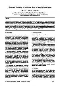
Figure 1. Snapshot of projectile-target interaction calculated using MPM. The projectile is colored red, while the target is colored green. Figure 1 shows a snapshot of a projectile-target interaction in an MPM calculation. The red material points represent the projectile, and the green material points represent the target. Initially all material points
4
were uniformly distributed in the projectile and in the target region. For this problem, if a Lagrangian mesh were used, mesh distortion would be a significant issue, especially near the material interface region. In an MPM calculation a stationary Eulerian mesh is used. The material points representing different materials move through the Eulerian mesh. The material points not only carry information about their position but also velocity, stress, material density and damage of the material. Since they are Lagrangian points, by incrementally updating the stress states on them, one can calculate the stress following the deformation history of the material and avoid the numerical diffusion issues associated with pure Eulerian calculation of the stress. With the stress calculated on material points, similarly to the finite element method, in MPM the momentum equation is solved based on virtual work theory, or weak solution of the governing equations (the material points play a role similar to the Gaussian integration points in a finite element calculation). The momentum equation (4) is solved as [4]
m il
u ilL − u iln = − ∑ vip ( σ ip + p g I ) ⋅ ∇ S l ( x ip ) + ( −θ i ∇ p g + f i + θ i ρ i g)Vl , Δt p =1
(8)
where superscript L denotes the Lagrangian step and superscript n denotes the time step, the summation is over all the material points representing phase i in the domain, vip and σip are respectively the volume and stress associated with material point p, Sl (xip ) is the shape function associated with node l , and
mil and Vl are respectively the mass of the phase i material on node l and the control volume associated with the node. The mass mil is calculated as
mil = ∑ mip Sl (xip ) ,
(9)
p =1
where mip is the mass of the phase i material on the material point p . The Lagrangian velocities calculated on the nodes are then interpolated to the material points as N
uipn +1 = uipn + ∑ uilL Sl (xip ) ,
(10)
l =1
where N is the total number of nodes in the problem domain. The positions of the material points are updated as N
xipn +1 = xipn + ∑ uilL Sl (xip )Δt .
(11)
l =1
Using this updated velocity and position of the material points the velocity at the node is updated as
uiln +1 = ∑ mip u np+1Sl (xipn +1 ) p =1
∑m p =1
ip
Sl (xipn+1 ) .
(12)
The process of updating the locations of the material points and then using the velocities on the material points to update the velocities on the nodes corresponds to the advection process in an Eulerian calculation. The numerical procedure described here is a direct extension of the material point method to multiphase flows. In multiphase flows, since there is more than one velocity field, the continuity condition (7) needs to be enforced to ensure there is not numerical material overlapping or artificial creation of voids between the materials. In a typical multiphase flow calculation using Eulerian methods, the continuity condition is enforced by finding pressures such that (7) is satisfied [2]. In MPM, the volume fractions are calculated as
θi =
1 Vl
∑v p =1
ip
Sl (xip ) ,
(13)
where vip is the volume of the material point p and Vl is the control volume associated with node l . There is an error of O[(Δx) d ] in this calculation of volume fraction, where d = 1 if there is a sharp material interface and d = 2 for a spatially smooth volume fraction. Therefore after summing such calculated volume fractions over all the phases, equation (7) cannot be satisfied exactly, and we can only have
5
M
M
∑ θi =∑ i =1
i =1
ρi
ρ ( pi ) 0 i
= 1 + O[(Δx) d ] .
(14)
If we use equation (7) to find a pressure increment Δp from time step n to n + 1 , it is equivalent to solving the following equation
fn+
∂f ∂f Δt + Δp = 1 , ∂t ∂p
where M
ρi
i =1
ρ ( pi )
f =∑
0 i
,
(15)
(16)
and f n denotes the function f evaluated at time step n . Since we can only calculate f n correctly within an error of O[(Δx) d ] , f n = 1 + O[(Δx) d ] , and the pressure increment solved from (15) then satisfies
⎡ ( Δx ) d ⎤ ∂f ∂f Δp + +O⎢ ⎥ = 0. ∂t ∂p Δt ⎣ Δt ⎦
(17)
In an explicit calculation, the time step Δt is proportional to Δx . If there is a sharp material interface in the calculation, d = 1 , and the error will be of zeroth order. In other words the computation will fail in the first time step. Indeed, we have used this approach to calculate a solid block translating through air with the same velocity as the air. Significant pressure change is observed in the numerical result while there should not be any. For a smoother field, although d = 2 , the error accumulation will also quickly lead to the failure of the calculation. Therefore for an MPM calculation, the continuity equation (7) cannot be used directly as in an Eulerian calculation. To overcome this difficulty of applying the MPM method to multiphase flows, in our calculation the continuity equation is enforced in the sense of the weak solution [5] as
∂⎛ m ⎞ ⎛ m ⎞ θ + u ⋅∇ θi ⎟ = 0 . ( ) ∑ ∑ i ⎟ m l ⎜ ⎜ ∂t ⎝ i =1 ⎠l ⎝ i =1 ⎠l
(18)
Although the sum of the volume fractions is not exactly one due to the discretization error, this equation ensures the error does not cause unphysical pressure changes in the pressure calculation, because the effect of the discretization error is largely offset by the second term in this equation. Equation (18) can be physically interpreted as, that following mixture motion the volume fraction sum is “incompressible”. 4.
Numerical Examples
The multi-material formulation and the extended material point method have been implemented in the CartaBlanca [4] numerical code. Figure 2 shows a CartaBlanca calculation of spalling of a porous solid caused by the impact of a flyer plate. In this calculation, both the top and the bottom plates are made of the same material, modeled as a linear elastic material until the tensile stress exceeds a limit to cause brittle failure. To illustrate the capability of the multi-pressure model, the air motion in the pores of the solid material and surrounding the solids is calculated. Although the effect of the air is negligible in this case, if the air is replaced by a viscous liquid, the effect of the liquid could be significant. We use air here to allow comparison with an analytical solution that ignores the air. Initially the thickness of the bottom plate is double that of the top plate, and the bottom plate is at rest while the top plate moves down at a speed of 100 m/s. Upon impact stress waves are generated on the impact surface and travel in both directions. These waves reflect back from the free surfaces as tension waves and meet on the middle plane in the bottom plate. The superposition of the tension waves doubles the tension stress and causes tensile failure in the brittle material. In Figure 2, damaged material is plotted in red. Without the effect of the air, the analytical result shows the spall time is about 1.18 μ s for this case, while our numerical calculation finds the spall time is about 1.12 μ s . The error is about 5%.
6
1.5
Y
1
0.5
0
0
0.5
1
X
Figure 2. Snapshot of a spalling process.
Figure 3. Snapshot of projectile-target interaction.
7
1.5
Figure 3 shows an example of large deformation. In this example a tungsten rod 5 cm in length and 0.4 cm in diameter is shot into a steel block with thickness 4.95 cm. The impact speed is 1.7 km/s. Figure 3 shows a snapshot of the tungsten rod penetrating the steel block. This example has been studied [9] using the Eulerian code CTH using the Johnson-Cook constitutive model [10] for both the tungsten rod and the steel block (with no fluid interaction). In our study the constitutive relations and material parameters are the same as those used in the CTH calculation. But differently from the CTH calculation, three velocity fields, for the tungsten, the steel and the air, are used to illustrate the capability of studying complicated fluid-structure interactions accompanied by large deformations. Figure 4 shows comparison between experimental data and our numerical results using different mesh sizes. Excellent agreement is observed.
11 10
Experiment (tail)
Tail position
Experiment (nose)
Height (cm)
9
Mesh size: 115x31
8
Mesh size: 230x62
7
Mesh size: 460x124
6 Upper steel surface
5 4 Nose position
3 2
Lower steel surface
1 0
0
10
20
30
40
50
60
70
Time (μs) Figure 4. Comparison of experimental data with computational results obtained using different mesh sizes.
In the two examples shown above the effect of gas is calculated although it is not really important. To show an example where gas interacts strongly with the surrounding structure, a calculation of interaction of an air blast and surrounding buildings is shown in Figure 5. In this example 5 kilotons of TNT are set off at the ground level of four buildings. Air shock interactions and the response of the buildings are calculated. The mechanical strength of the buildings is considered. In the figure, a crater and building damage are evident. Although the initial conditions and building properties are fictitious, the results show the modeling capability introduced by the combination of the multi-material formulation and the extended material point method.
8
Figure 5. Effects of air blast on high rise buildings. The strength of the buildings is considered.
5.
Conclusions
A recently developed multi-pressure, multi-material deformation model for continuous multiphase flows has been implemented in the CartaBlanca [4] numerical code. Combination of an advanced version of the material point method and the continuous multiphase flow model has been shown to significantly enhance capability in studying fluid-structure interaction problems, especially for large deformations. Examples calculated using the multiphase flow model and the enhanced MPM method show satisfactory comparison with theoretical and experimental results.
6.
Acknowledgement
This work was performed under the auspices of the United States Department of Energy with support from the Army Research Office. References
1.
F.L. Addessio, J. R. Baumgardner, J. K. Dukowicz, N. L. Johnson, B. A. Kashiwa, R. M. Rauenzahn, C. Zemach, CAVEAT: A Computer Code for Fluid Dynamics Problems with Large Distortion and Internal Slip, Los Alamos National Laboratory Report LA-10613-MS, Rev. 1, May, 1992.
2.
A. Prosperetti, G. Tryggvason, Computational Methods for Multiphase Flow, Chapter 10, Cambridge University Press (2006).
9
3.
D.Z. Zhang, W. B. VanderHeyden, Q. Zou, N. T. Padial-Collins, Pressure calculations in disperse and continuous multiphase flows, Int. J. Multiphase Flow 33, 86 (2007).
4.
http://www.lanl.gov/projects/CartaBlanca/
5.
http://www.lanl.gov/projects/CartaBlanca/webdocs/VolFracAlg.pdf
6.
D. Sulsky, S.-J. Zhou, H. L. Schreyer, Application of a particle-in-cell method to solid mechanics, Computer Physics Communication 87, 236 (1995).
7.
F.H. Harlow, The particle-in-cell computing method for fluid dynamics, Methods Comput. Phys. 3, 219 (1963).
8.
F.H. Harlow, A.A. Amsden, Fluid Dynamics, A LASL Monograph, Los Alamos National Laboratory Report LA-4700, 1971.
9.
C. E. Anderson, V. Hohler, J. D. Walker, A. J. Stilp, Time-Resolved Penetration of Long Rods into Steel Targets, Int. J. Impact Engng. 16 (1), 1 (1995).
10. G. R. Johnson, W. H. Cook, Fracture characteristics of three metals subjected to various strains, strain rates, temperatures and pressures, Engng. Fracture Mechanics 21 (1), 31 (1985).
10