SIMULATION OF STEADY-STATE AND DYNAMIC BEHAVIOUR OF A TUBULAR CHEMICAL REACTOR Petr Dostál, Vladimír Bobál, and Jiří Vojtěšek Department of Process Control, Faculty of Applied Informatics Tomas Bata University in Zlin Nad Stráněmi 2911, Zlín 760 05, Czech republic E-mail:
[email protected]
KEYWORDS Tubular chemical reactor, mathematical model, steadystate, dynamics. ABSTRACT The paper presents some results concerning analysis and simulation of steady-state and dynamic behaviour of a tubular chemical reactor. This analysis represents a necessary condition for the reactor control design purposes. The mathematical models used in simulations together with simulation results are contained.
MODEL OF THE PLANT An ideal plug-flow tubular chemical reactor with a k1
k2
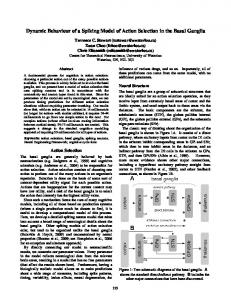
simple exothermic consecutive reaction A → B → C in the liquid phase and with the countercurrent cooling is considered as shown in Fig. 1. qc, Tc out
qc, Tc L
qr, Tr 0
qr, Tr out
ci 0
ci out
INTRODUCTION Tubular chemical reactor are units frequently used in chemical and biochemical industry. From the system theory point of view, tubular chemical reactors belong to a class of nonlinear distributed parameter systems. Their mathematical models are described by sets of nonlinear partial differential equations (PDR). The methods of modelling and simulation of such processes are described eg. in (Luyben 1989; Ingham et al. 1994; Severance 2001; Babu 2004). Relations between process behaviour and their control methods can be found in (Seborg et al. 1989; Ogunnaike and Ray 1994; Marlin 1995; Corriou 2004). It is well known that the control of chemical reactors, and, tubular reactors especially, often represents very complex problem. The control problems are due to the process nonlinearity, its distributed nature, and high sensitivity of the state and output variables to input changes. In addition, the dynamic characteristics may exhibit a varying sign of the gain in various operating points, the time delay as well as non-minimum phase behaviour. Evidently, the process with such properties is hardly controllable by conventional control methods, and, its effective control requires application some of advanced methods (e. g. Adaptive Control, Predictive Control, Robust Control or any others). However, at all events, a previous analysis of the process behaviour is obligatory. The paper presents all mathematical models used for simulations of both steady-state and dynamic charakteristics of the tubular chemical reactor together with results of some simulations. The combinations of observed variables are chosen in accordance with purposes of prospective control design. Proceedings 22nd European Conference on Modelling and Simulation ©ECMS Loucas S. Louca, Yiorgos Chrysanthou, Zuzana Oplatková, Khalid Al-Begain (Editors) ISBN: 978-0-9553018-5-8 / ISBN: 978-0-9553018-6-5 (CD)
z L
Figure 1: Tubular chemical reactor. Heat losses and heat conduction along the metal walls of tubes are assumed to be negligible, but dynamics of the metal walls of tubes are significant. All densities, heat capacities, and heat transfer coefficients are assumed to be constant. Under above assumptions, the reactor model can be described by five PDRs in the form ∂c A ∂c A + vr = − k1 c A ∂t ∂z
(1)
∂c B ∂c B + vr = k1 c A − k 2 c B ∂t ∂z ∂T r ∂T Qr 4U 1 + vr r = − (T − T w ) ∂t ∂ z (ρc p ) r d 1 (ρc p ) r r ∂T w ∂t
=
4 (d 22
− d 12 ) (ρc p ) w
⎣⎡ d 1U 1 (T r − T w ) +
(2) (3)
(4)
+ d 2 U 2 (Tc − T w ⎤⎦
∂T c ∂t
− vc
∂T c ∂z
=
4 n1 d 2 U 2 (d 32
− n1 d 22 ) (ρc p ) c
(T w − Tc ) (5)
with initial conditions c A ( z ,0) = c As ( z ) , c B ( z ,0) = c Bs ( z ) , Tr ( z ,0) = Trs ( z ) ,
Tw ( z ,0) = Tws ( z ) , Tc ( z ,0) = Tcs ( z ) and boundary conditions c A (0, t ) = c A0 (t ) , c B (0, t ) = c B 0 (t ) , Tr (0, t ) = Tr 0 (t ) ,
control variables, whereas other inputs enter into the process as disturbances. As the controlled output, next to c B out also the mean reactant temperature given by
Tc ( L, t ) = Tc L (t ) .
Here, t is the time, z is the axial space variable, c are concentrations, T are temperatures, v are fluid velocities, d are diameters, ρ are densities, cp are specific heat capacities, U are heat transfer coefficients, n1 is the number of tubes and L is the length of tubes. The subscript (⋅)r stands for the reactant mixture, (⋅)w for the metal walls of tubes, (⋅)c for the coolant, and the superscript (⋅)s for for steady-state values. The reaction rates and heat of reactions are nonlinear functions expressed as ⎛−Ej ⎞ ⎟ , j = 1, 2 k j = k j 0 exp ⎜⎜ ⎟ R T r ⎝ ⎠ Q r = (−ΔH r1 ) k 1 c A + (−ΔH r 2 ) k 2 c B
(7)
where k0 are pre-exponential factors, E are activation energies, ( - ΔHr) are in the negative considered reaction entalpies, and R is the gas constant. The fluid velocities are calculated via the reactant and coolant flow rates as vr =
4 qr π n1 d 12
, vc =
4 qc 2
2
π ( d 3 − n1 d 2 )
(8)
The parameter values with correspondent units used for simulations are given in Table 1. Table 1: Parameter values
d1 = 0.02 m
d2 = 0.024 m d3 = 1 m
ρr = 985 kg/m3 3
ρw = 7800 kg/m 3
ρc = 998 kg/m
2
U1 = 2.8 kJ/m s K 16
k10 = 5.61⋅10 1/s E1/R = 13477 K
0
Tr ( z , t ) d z
(9)
COMPUTATION MODELS
For computation of both steady-state and dynamic characteristics, the finite diferences method is employed. The procedure is based on substitution of the space interval z ∈< 0, L > by a set of discrete node
{ z i } for
i = 1, … , n ,and, subsequently, by
approximation of derivatives with respect to the space variable in each node point by finite differences. Two types of finite differences are applied, either the backward finite difference ∂ y( z, t ) ∂z
≈
y ( z i , t ) − y ( z i −1, t ) h
z=zi
=
y (i, t ) − y (i − 1, t ) (10) h
=
y (i + 1, t ) − y (i, t ) . (11) h
or the forward finite difference ∂ y ( z, t ) ∂z
y ( z i +1 , t ) − y ( z i , t )
≈
h
z=zi
Here, a function y ( z , t ) is continuously differentiable in < 0, L > , and, h = L n is the diskretization step. Dynamic Model
cpr = 4.05 kJ/kg K
d c B (i )
cpw = 0.71 kJ/kg K
dt
= k 1 (i ) c A (i ) − ⎣⎡b 0 + k 2 (i ) ⎦⎤ c B (i ) +
2
U2 = 2.56 kJ/m s K 18
k20 = 1.128⋅10 1/s E2/R = 15290 K
(-ΔHr1) = 5.8⋅104 kJ/kmol (-ΔHr2) = 1.8⋅104 kJ/kmol From the system engineering point of view, c A ( L, t ) = c A out , c B ( L, t ) = c B out , T r ( L, t ) = T r out and T c (0, t ) = T c out are the output variables, and, q r (t ) ,
dT r (i ) dt
= b1 Q r (i ) − (b 0 + b 2 ) T r (i ) + b 0 T r (i − 1) +
(14)
+ b 2 T w (i )
dT w (i ) dt
= b3 ⎡⎣T r (i ) − T w (i ) ⎤⎦ + b 4 ⎡⎣T c (i ) − T w (i ) ⎤⎦ (15)
dT c (m) dt
= −(b5 + b 6 ) T c (m) + b5 T c (m + 1) +
(16)
+ b 6 T w ( m)
are the input
variables. Among them, for the control purposes, mostly q r (t ) and q c (t ) can be taken into account as the
(13)
+ b 0 c B (i − 1)
cpc = 4.18 kJ/kg K
q c (t ) , c A 0 (t ) , T r 0 (t ) and T c L (t )
L
Applying the substitutions (10), (11) in (1) – (5) and, omitting the argument t in parenthesis, PDRs (1) – (5) are approximated by a set of ODRs in the form d c A (i ) = − ⎡⎣b 0 + k 1 (i ) ⎤⎦ c A (i ) + b 0 c A (i − 1) (12) dt
n1 = 1200
L=8m
∫
can be under some assumptions considered.
points (6)
1 L
Tm (t ) =
for i = 1, ... , n conditions
and
m = n − i + 1 , and, with initial
s
s
c A (i, 0) = c A (i ) ,
⎛ −E j ⎞ s ⎟ , j = 1, 2 k j (i ) = k j 0 exp ⎜ ⎜ RT s (i ) ⎟ ⎝ r ⎠
s
c B (i,0) = c B (i ) ,
T r (i, 0) = T r (i ) ,
T w (i, 0) = T ws (i ) and T c (i, 0) = T cs (i ) for i = 1, ... , n .
The boundary conditions enter into Eqs. (12) – (14) and (16) for i = 1 . Now, nonlinear functions in Eqs. (12) – (16) take the discrete form ⎛ −E j ⎞ k j (i ) = k j 0 exp ⎜ , j = 1, 2 ⎜ RT (i ) ⎟⎟ ⎝ r ⎠ Q r (i ) = (−ΔH r1 ) k 1 (i ) c A (i ) + (−ΔH r 2 ) k 2 (i ) c B (i )
b5 =
vc h
, b6 =
2
2
(d 2 − d 1 ) (ρc p ) w 4 n1 d 2 U 2
(d 32 − n1 d 22 ) (ρc p ) c
(19)
1 n
.
s
∑ T (z , t)
(20)
i
i =1
Computation of the steady-state characteristics is necessary not only for a steady-state analysis but the s
steady state values y (i ) also constitute initial conditions in ODRs (12) – (16) (here, y presents some of the variable in the set (12) – (16)). The steady-state model can simply be derived equating the time derivatives in (12) – (16) to zero. Then, after some algebraic manipulations, the steady-state model takes the form of difference equations
c Bs (i ) =
b0 +
1 b0 +
k 2s (i )
s k 1 (i )
c As (i − 1)
⎡ k s (i ) c s (i ) + b c s (i − 1) ⎤ (22) 0 B A ⎣ 1 ⎦
1 ⎡ s s b T (i ) + b 4 Tc (i ) ⎤ = ⎦ b3 + b 4 ⎣ 3 r
(24)
q c = 0.35 and
s
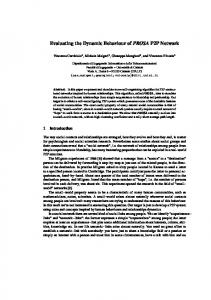
peak on the reactant B profile is given by considered reaction type. The existence of a maximum on the reactant temperature profile (so called hot spot) is a common property of many tubular reactors with exothermic reactions. The concentration and reactant profiles for various values q cs are exhibited in Figs. 4 – 6. All simulation results document strong dependence of all profiles upon this input in the steady-state. The dependences of some output variables upon s s q c and for various q r are shown in Figs. 7 – 9. The
courses document strong sensitivity of outputs upon both flow rates which can be considered as control inputs. In this way obtained results are very important for the reactor control design. The dependence of the component B concentration 3.0 2.5 2.0 1.5 1.0
s
cA
0.5
s
cB
0.0
1 ⎡ s s s T c ( m) = b T (m + 1) + b 6 T w (m) ⎤ ⎦ b5 + b 6 ⎣ 5 c for i = 1, ... , n and m = n − i + 1 , and, functions accordant with a steady-state are
s
s
T c 0 = 299 ,
q r = 0.15 are shown in Figs. 2, 3. The presence of a
(21)
1 ⎡ s s s b Q (i ) + b 0 T r (i − 1) + b 2 T w (i ) ⎤ (23) ⎦ b0 + b 2 ⎣ 1 r s T w (i )
s
s
s
T r (i ) =
b0
Steady-state characteristics were computed from Eqs. (21) – (27) using fixed point iterations algorithm and for n = 200. Typical concentration and temperature profiles c B 0 = 0 , T r 0 = 323 ,
Steady-State Model
c As (i ) =
(28)
i =1
s
n
r
s (zi ) r
along the reactor tubes computed for c A 0 = 2.85 ,
Here, the formula for computation of Tm (9) is rewriten to the discrete form Tm (t ) =
∑T
Steady-state Characteristics
3
2
4d 2 U 2
n
The combinations of the inputs and outputs in all simulations of steady-state and dynamic characteristics were considered with respect to an importantance for a prospective control design.
s
2
(d 2 − d 1 ) (ρc p ) w
, b4 =
1 n
SIMULATION RESULTS
cA, cA (kmol / m )
4 d 1U 1
Here, the formula for computation Tm takes the form
(17)
for i = 1, … , n. The parameters b in Eqs. (12) – (16) are calculated from formulas v 4U 1 1 b 0 = r , b1 = , b2 = , (ρc p ) r h d 1 (ρc p ) r b3 =
Q rs (i ) = (−ΔH r1 ) k 1s (i ) c As (i ) + (−ΔH r 2 ) k 2s (i ) c Bs (i ) (27)
T ms =
(18)
(26)
(25)
nonlinear
0
1
2
3
4 z (m)
5
6
7
8
Figure 2: Concentration profiles along the reactor.
s
c B out on the reactant mean temperature is presented in 1.2
Temperatures (K)
s
3
0.4
qr = 0.1
0.2
s
0.0
s
Tw s
Tc
330
s
qr = 0.15
0.6
Tr
340
s
qr = 0.2
0.8
s
350
s
qr = 0.25
1.0
cA out (kmol/m )
Fig. 10. Also this result can be important when the output concentration cB is non-measurable and, its desired (maximum) value could be achieved only by measured reactant temperatures along the reactor.
0.20
Hot spot
320
0.25
0.30
0.35 0.40 s 3 qc (m /s)
0.45
0.50
s
Figure 7: Dependence of c A out on q cs for various q rs .
310 300 0
1
2
3
4 5 z (m)
6
7
s
8
3.0
3
s
2.5
s
s
qr = 0.2
3
cB out (kmol/m )
Figure 3: Temperature profiles along the reactor.
cA (kmol/m )
qr = 0.25
2.0
2.0
1.5 s
1.0
qr = 0.1
0.5
qr = 0.15
s
0.0
1.5 s
0.20
qc = 0.5
1.0 0.5
s qc
s
qc = 0.2
0.0 0
1
s qc
= 0.3
0.25
0.30
= 0.4
0.35 0.40 s 3 qc (m /s)
0.45
0.50
s
2
3
4 z (m)
5
6
7
Figure 8: Dependence of c B out on q cs for various q rs .
8
Figure 4: Concentration c As profiles for various q cs . 348 344 340
= 0.4 s
1.5
qc = 0.5
1.0
s
3
cB (kmol/m )
s qc
Tm (K)
2.0
s
s
0.5
336 332 328
qc = 0.3
0
1
2
3
Figure 5: Concentration
s
qr = 0.25 s qr = 0.1
324 0.20
4 z (m)
c Bs
5
6
7
0.25
8
profiles for various
q cs
.
0.30
0.35 0.40 s 3 qc (m /s)
0.45
0.50
Figure 9: Dependence of T ms on q cs for various q rs . 2.5
370 365 360 355 350 345 340 335 330 325 320
s
qc = 0.2
2.0
3
cB out (kmol/m )
s
qc = 0.3 s
qc = 0.4 s
s
s
s
qr = 0.2
s
qc = 0.2
0.0
Tr (K)
s
qr = 0.15
qc = 0.5
1.5 1.0 0.5 0.0
0
1
2
3
4 z (m)
5
6
7
8
325 s
Figure 6: Reactant temperature profiles for various q c .
330
335 s Tm (K)
340
345
Figure 10: Dependence of c Bs upon T ms .
Dynamic Characteristics
All dynamic charakteristics were computed using the Runge-Kutta method with a fixed step. All inputs and outputs were considered as deviations from their steady values. This form is frequently used in the control. The deviations are denoted as follows:
0.8 0.4 3
y1 (kmol/m )
v1 (t ) = q c (t ) − q cs v 2 (t ) =
As an influence illustration of the random disturbances on the process output, the responses to random signals cA0 and Tr0 are shown in Figs. 15 – 18. These simulation results document high sensitivity of both outputs to random input signals.
s c A0 (t ) − c A 0 s
v 3 (t ) = T r 0 (t ) − T r 0 s c B out (t ) − c B out
y1 (t ) =
-0.8
0
s
s
s
s
0.0
-0.4 v1 = - 0.075 v1 = - 0.15
-0.8 -1.2
v2 = 0.25
0 -4 -8
v2 = - 0.25 v2 = - 0.5
-16 0
20
40
20
40
60
3
0.5 0.0 -0.5 -1.0
80 100 120 140 160 180 t (s)
Figure 11: Output concentracion cB step responses. 20 16 12 8 4 0 -4 -8 -12 -16
y1 v2
0
0
20
40
60
v1 = 0.075
100
150 t (s)
200
250
300
y2
4 y2, v3 (K)
y2 (K)
v1 = 0.15
50
Figure 15: Output cB response to random input v2.
v1 = - 0.15 v1 = - 0.075
80 100 120 140 160 180 t (s)
1.0
-1.5
0
60
Figure 14: Mean temperature step responses.
y1, v2 (kmol/m )
3
y1 (kmol/m )
v1 = 0.075
v2 = 0.5
-12
v1 = 0.15
0.4
80 100 120 140 160 180 t (s)
4
The responses to qc and cA0 step changes in Figs. 11-14 clearly document a strong nonlinearity of the process. Moreover, they show a better applicability of the reactant mean temperature as the controlled output in comparison with the output concentration cB having in this regard very unfavourable properties.
0.8
60
8
and
T c 0 = 299 .
40
12
y2 (K)
T r 0 = 323
20
v2 = 0.25
Figure 13: Output concentracion cB step responses.
steady-state values computed from the model (21) – (25) for the input steady-state values q rs = 0.15 c A 0 = 2.85 ,
v2 = 0.5
-1.2
c B out = 1.345 and T ms = 337.77 are the output
q cs = 0.25 ,
v2 = - 0.5
-0.4
y 2 (t ) = T m (t ) − T ms
where
v2 = - 0.25
0.0
v3
2 0
-2 -4
80 100 120 140 160 180 t (s)
Figure 12: Mean temperature Tm step responses.
0
50
100
150 t (s)
200
250
300
Figure 16: Output Tm responses to random input v3.
REFERENCES
3
v2 (kmol/m )
0.6 0.4 0.2 0.0 -0.2 -0.4 -0.6
y2 (K)
8 6 4 2 0 -2 -4 -6 0
50
100
150 t (s)
200
250
300
Figure 17: Output Tm responses to random input v2.
AUTHOR BIOGRAPHIES
v3 (K)
3 2 1 0 -1 -2 -3
0.8 3
y1 (kmol/m )
Luyben, W.L. 1989. Process modelling, simulation and control for chemical engineers. McGraw-Hill, New York. Ingham, J.; I. J. Dunn; E. Heinzle; and J. E. Přenosil. 1994. Chemical Engineering Dynamics. Modelling with PC Simulation. VCH Verlagsgesellschaft, Weinheim. Severance, F.L. 2001. System Modeling and Simulation. Wiley, Chichester. Babu, B.V. 2004. Process Plant Simulation. Oxford University Press, New Delhi. Ogunnaike, B.A., Ray, W.H.: Process dynamics, modeling, and control. Oxford University Press, New York, 1994. Seborg, D.E; T.F. Edgar; and D.A. Mellichamp. 1989. Process Dynamics and Control. Wiley, Chichester. Marlin, T.E.: Process control. Designing processes and control systems for dynamic performance. McGraw-Hill, New York, 1995. Corriou, J.-P. 2004. Process Control. Theory and Applications. Springer – Verlag, London.
0.4 0.0
-0.4 -0.8 0
50
100
150 t (s)
200
250
300
Figure 18: Output concentration cB response to random input v3. CONCLUSIONS
In the paper, the mathematical model of a tubular chemical reactor with a consecutive exothermic reaction has been presented. The computer models for simulations of steady-state and dynamic characteristics in the form of sets of ordinary differential and difference equations were derived to an original model in the form of partial differential equations The simulation experiments were chosen with a view to a prospective control of the process. ACKNOWLEDGMENTS
This work was supported in part by the Ministry of Education of the Czech Republic under the grant MSM 7088352101 and by the Grant Agency of the Czech Republic under the grant No. 102/06/1132.
PETR DOSTÁL was born in Kněždub, Czech Republic in 1945. He studied at the Technical University of Pardubice, where he obtained his master degree in 1968 and PhD. degree in Technical Cybernetics in 1979. In the year 2000 he became professor in Process Control. He is now head of the Department of Process Control, Faculty of Applied Informatics of the Tomas Bata University in Zlín. His research interest are modeling and simulation of continuous-time chemical processes, polynomial methods, optimal and adaptive control. You can contact him on email address
[email protected] VLADIMÍR BOBÁL was born in Slavičín, Czech Republic in 1942. He graduated in 1966 from the Brno University of Technology. He received his Ph.D. degree in Technical Cybernetics at Institute of Technical Cybernetics, Slovak Academy of Sciences, Bratislava, Slovak Republic. He is now Professor in the Department of Process Control, Faculty of Applied Informatics of the Tomas Bata University in Zlín. His research interests are adaptive control systems, system identification and CAD for self-tuning controllers. You can contact him on email address
[email protected] JIŘÍ VOJTĚŠEK was born in Zlin, Czech Republic and studied at the Tomas Bata University in Zlin, where he got his master degree in chemical and process engineering in 2002 and finished his Ph.D. in Technical Cybernetics in 2007. He works as a senior lecturer in the Department of Process Control, Faculty of Applied Informatics, Tomas Bata University in Zlin. You can contact him on email address
[email protected].