Simulation of Storm Occurrences Using Simulated Annealing

4394

JOURNAL OF CLIMATE

VOLUME 18

Simulation of Storm Occurrences Using Simulated Annealing RAVINDRA S. LOKUPITIYA Department of Atmospheric Science, Colorado State University, Fort Collins, Colorado

LEON E. BORGMAN L. E. Borgman, Inc., Laramie, Wyoming

RICHARD ANDERSON-SPRECHER Department of Statistics, University of Wyoming, Laramie, Wyoming (Manuscript received 4 February 2004, in final form 6 April 2005) ABSTRACT Modeling storm occurrences has become a vital part of hurricane prediction. In this paper, a method for simulating event occurrences using a simulated annealing algorithm is described. The method is illustrated using annual counts of hurricanes and of tropical storms in the Atlantic Ocean and Gulf of Mexico. Simulations closely match distributional properties, including possible correlations, in the historical data. For hurricanes, traditionally used Poisson and negative binomial processes also predict univariate properties well, but for tropical storms parametric methods are less successful. The authors determined that simulated annealing replicates properties of both series. Simulated annealing can be designed so that simulations mimic historical distributional properties to whatever degree is desired, including occurrence of extreme events and temporal patterning.

1. Introduction Hurricanes are among the most destructive forces in nature. Strong winds and storm surges associated with landfall hurricanes cause intensive damage to human life and property along coastal areas in the United States. In 1992, when Hurricane Andrew struck the coast of Florida it caused over $30 billion in direct economic losses. As human population increases worldwide, densely populated cities also tend to grow toward high hazard areas, increasing the risk of damage due to future occurrences. The modeling of hurricane frequencies is consequently of great interest for risk assessment and associated planning. Traditionally, annual hurricane occurrences are modeled using parametric models. Poisson and negative binomial distributions are two competing probability

Corresponding author address: Dr. Ravindra S. Lokupitiya, Department of Atmospheric Science, Colorado State University, Fort Collins, CO 80523. E-mail: [email protected]

© 2005 American Meteorological Society

JCLI3546

models that have been used successfully to represent annual numbers of events (Chen et al. 2004). Observed data fit well with these distributions, but there are questions about how to best project observed results into the future, in part because of slight temporal patterning in existing data. One way to maintain patterning is to incorporate autocorrelations, requiring simulation of correlated Poisson distributions. Alternatively, a deterministic (probably nonlinear) trend successfully removes apparent correlations, but extrapolation of any such trend is open to question. To improve on such representations, much research has been done in the area of modeling hurricane occurrences during the last decade. Gray et al. (1992) introduced a method to predict seasonal hurricane activity during the June to November hurricane season. Seven indices of Atlantic seasonal tropical storm activity, including frequency, were considered as responses regressed onto the predictor variables wind and rainfall. Parameter estimation was done using the jackknife procedure, with the intent of ensuring that the prediction for any year is independent of the observation for that

1 NOVEMBER 2005

LOKUPITIYA ET AL.

year. Elsner and Schmertmann (1993), however, argue that Gray’s procedure is not fully independent, and they provide a fully cross-validated alternative. Elsner and Bossak (2001) developed a Bayesian approach to predict hurricane occurrences. They combined more accurate hurricane records during the twentieth century with less accurate accounts from the nineteenth century to produce a better estimate for the posterior distribution of the annual rates. Elsner and Jagger (2004) further improve this method using an hierarchical Bayesian approach incorporating effects of the El Niño–Southern Oscillation (ENSO) and the North Atlantic Oscillations (NAOs) as covariates. Parameter estimation of the posterior distribution was done using Markov Chain Monte Carlo (MCMC) technique. Chen et al. (2003, 2004) described a hurricane simulation system built on a three-tier system architecture design. They compared both existing parametric methods, the Poisson and negative binomial distributions, and selected a final model using a chi-square statistic. As computing power and availability have increased, simulation has become a standard tool for determining properties of data, the performance of new methodologies, and the prediction of possible timelines of future events. Frequently, needed simulations should replicate fundamental characteristics of some set of existing data, such as a historical hurricane record. Simulations are most often model based, as opposed to data based, in which case historical data are only used to establish parameters in the assumed parametric model. The methods previously described for modeling hurricane occurrences are not as appropriate for simulation of other series with atypical distributions, such as tropical storms. Nonparametric methods such as kernel density estimation can be used, but such nonparametric methods typically require a large historical dataset in order to perform adequately. Liu and Taylor (1990) described a nonparametric density estimation technique when observations are contaminated with random noise, utilizing Fourier and kernel function estimation methods. Another potential problem with historical data is the possibility of temporal patterning. Patterning may take the form of trends, cycles, or autocorrelations. Most data simulation methods assume independent identically distributed observations. Hart (1984) considered properties of density estimators used with data generated by an AR(1) process and found substantial deterioration of efficiency. Standard methods may not apply when numbers are correlated and may not be suitable for simulations. When marginal distributions are of a known parametric form, many approaches exist for simulating pseudorandom numbers with desired patterns of auto-

4395

correlation. For example, in standard time series analysis, realizations of known Gaussian Auto-Regressive Integrated Moving Average (ARIMA) processes can be readily simulated. More generally, Polge et al. (1973) present a procedure, based on correlation transfer, to generate a pseudorandom set with a selected distribution and correlation. After selecting a sample from the desired distribution, sample values are rearranged until the desired correlation is achieved. However, the rearrangements are limited, and the method works well only when samples are large. Also, the method is not suitable to generate pseudorandom numbers with a specific correlation structure. Lakhan (1981) found a fast method to generate autocorrelated pseudorandom numbers with specific distributions. First, standard normal correlated random numbers with the desired correlation structure are simulated; then these random numbers are transformed into correlated uniform variates by using the probability integral transformation Ut ⫽ ⌽(Xt). Finally, to simulate correlated random numbers from other distributions, correlated U(0, 1) random numbers are simulated as described above and the inverse transformation X ⫽ F⫺1(Y ) is used to produce values with the desired marginal distributions. Both methods described are restricted to a parametric setting. The method of Polge et al. could perhaps be extended to a distribution known only from a single dataset by a modified bootstrap approach: a random sample could be drawn from the empirical distribution of the sample data (bootstrapping) and values could be rearranged until correlations approach sample values, but the limitations cited above still exist. When data consist of a series of random numbers but we know neither the underlying distribution nor the underlying correlation structure, improved methods are needed. An adaptation of simulated annealing may be used to this end. In this paper, we describe a nonparametric approach based on the simulated annealing algorithm to simulate future occurrences of events such as hurricanes and tropical storms, based on historical records. Our method accounts for dominant distributional properties in historical series without reverting to parametric modeling and may also be designed to reflect temporal patterning present in the historical storm records. In the case of hurricanes and tropical storms, temporal patterns are subtle and may be explained in different ways, but our method has the virtue of accounting for such patterns in whatever way the practitioner believes best. The form that we describe does not incorporate covariates such as time functions, but the procedure can easily be extended to this case if covariate values are known,

4396

JOURNAL OF CLIMATE

forecast, or simulated. The method is flexible enough to enforce nearly any desired degree of similarity to the original data. Simulated annealing has found successful application in a variety of forms and for a variety of applications. Deutsch (1996) described a method that simulates histograms and two-variable scatterplots using the simulated annealing algorithm. However, his method does not account for autocorrelation in the original data. Application of simulated annealing in oceanography and meteorology is widely available. Barth and Wunsch (1990) used simulated annealing to optimize the oceanographic experiment design problem. The problem of obtaining oceanographic observations, which is both difficult and costly, has been a challenging task for oceanographers since earliest days. The objective in this case is to locate efficient grid locations to take measurements for a given model. Krüger (1993) used simulated annealing to optimize a cost function in data assimilation. This method is applied to find a steady-state optimum of a nonlinear time-dependent model fitted to real observations. According to his comparison, the simulated annealing is robust and converges to a solution, whereas the sophisticated adjoint technique fails. He also found that the annealing procedure is capable of handling problems with many degrees of freedom. Other applications of simulated annealing in data assimilation include the work of Krüger (1993), Bennett and Chua(1994), and Pathmathevan et al. (2003). The version of simulated annealing described in the literature that is perhaps closest to the form shown here is that of Goovaerts (1997), who simulated geostatistical data using the simulated annealing algorithm. He used an objective function to reproduce features of a given semivariogram model. The method described below simulates data in a single (time) dimension, not only forcing the second-order moments seen in the semivariogram but also forcing the third- and fourthorder moments of the original series. In principle the method should also be applicable for data correlated in multiple dimensions.

2. Simulated annealing Simulated annealing, also known as Monte Carlo annealing, statistical cooling, probabilistic hill climbing, stochastic relaxation, or the probabilistic exchange algorithm, has attracted significant attention as a suitable choice for optimization problems of very large scale (van Laarhoven and Aarts 1987). The unusual name was chosen because of analogs that exist between simulated annealing and thermodynamics, specifically with the way that liquids freeze and crystallize or metals cool and anneal (Press et al. 1990).

VOLUME 18

When the temperature of a liquid increases, the molecules of the liquid can move freely with respect to one another. If the liquid is cooled slowly near the freezing point, thermal mobility is lost and the atoms line themselves up to form a crystal. This crystal is the state of minimum energy for the system. The keynote of the procedure is slow cooling, allowing enough time for redistribution of the atoms as they lose mobility. This physical description has precise counterparts in the optimization method called simulated annealing. Descriptions of the mathematical algorithm often lean on the language of the physical analog, and we freely revert to this metaphor in the outline below. Given a temperature value T, the system will reach thermal equilibrium, characterized by a probability of being in a state with energy E given by the Boltzmann distribution, prob共E兲 ⬃ exp

冉 冊

⫺E , kT

where k is the Boltzmann constant. When the temperature is decreased gradually, the Boltzmann distribution approaches a state with lowest energy, and, finally, when the temperature reaches zero, only the minimum energy states have nonzero probability of occurrence. However, when cooling is rapid, the system will not reach the thermal equilibrium for each temperature value and will finally reach one of many metastable amorphous structures rather than the low energy crystalline lattice structure. In an optimization problem, reaching an undesirable amorphous state corresponds to stabilization at a local minimum, but not a global minimum, of the objective function. Even with a low temperature, a system may be in a high-energy state. Hence, there is a corresponding chance for the system to jump from a local energy minimum to a more global one. The system sometimes goes uphill as well as downhill, but the lower the temperature; the less likely there will be any significant uphill deviation. Metropolis et al. (1953) incorporated these principles into numerical calculations. A system changes its state from energy E1 to energy E2 with probability p ⫽ min{exp[⫺(E2 ⫺ E1)/kT ], 1}. When E2 ⬍ E1, this probability is p(·) ⫽ 1. In other words, with E2 ⬍ E1, one always moves to a new state, and otherwise a new state is entered with probability p. For other than thermodynamic systems the Metropolis algorithm may be altered so that configurations assume the role of the states of a solid, while the objective function (obj) takes the role of energy. Thus reaching the minimum energy level of the system is equivalent to reaching the global minimum of the objective function.

1 NOVEMBER 2005

LOKUPITIYA ET AL.

4397

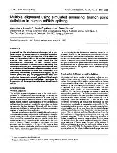
FIG. 1. Flowchart of the simulated annealing algorithm.

The steps in the algorithm are as follows: (i) Initialize (initial “temperature” and configuration). (ii) Choose a new configuration. (iii) Accept the new configuration if it minimizes the objective function (obj). (iv) Return to (ii) until the equilibrium criterion is satisfied, then reduce the temperature. (v) Check whether the system is “frozen.” If it is, stop the procedure; otherwise return to step (ii). Choosing an initial value for temperature (T0) requires some experimentation. We suggest generating some random rearrangements of configurations and determining the differences of objective functions encountered from move to move. The initial value for temperature is chosen as a considerably larger number than the largest difference between the objective functions. However, the choice of suitable value for T0 is highly problem dependent. A good approximation can be empirically found such that the initial acceptance probability is 0.8. When the system is frozen, the objective function

cannot be minimized any further. At this stage, if we iterate the procedure by reducing the temperature further, the objective function stays constant. In most cases for which simulated annealing is worth the effort, the objective function is multimodal within the domain of interest. Unlike simulated annealing, most other optimization procedures tend to stop at the first minimum encountered and cannot be easily used for finding the global minimum. A flowchart of the algorithm is given in Fig. 1.

3. Nonparametric correlated data simulation using simulated annealing Simulated annealing is particularly useful when one has need of data simulations without referring to a parametric model. The goal is to simulate a series of occurrences that mimics desired distributional properties, including correlation structure, of a known dataset. For distributions that do not readily fit a parametric form, a natural criterion for data fit is agreement with sample moments. Autocorrelations (whether with re-

4398

JOURNAL OF CLIMATE

spect to time, space, or some other measure) can be measured using conventional pairwise correlations for different lags or, as is done in spatial data analysis, using the semivariogram (Cressie 1993). For a stochastic process {X(t); t ∈ D}, indexed over time, the semivariogram has definition 1⁄2var[X(t1) – X(t2)] ⫽ ␥(|t1 – t2|), for all t1, t2 ∈ D. When {X(t): t ∈ D} satisfies E[X(t)] ⫽ ␮, for all t ∈ D, the relationship between the covariance function (covariogram), C(␶) ⫽ cov[X(t ⫹ ␶), X(t)], and the semivariogram is given by ␥(␶) ⫽ [C(0) ⫺ C(␶)] ⫽ C(0)(1 ⫺ R(␶)), where R(␶) is the autocorrelation function. Any time series problem can be thought of as a one-dimensional spatial problem, and we use the semivariogram approach to optimize properties of a particular time series simulation. The semivariogram could be replaced, if desired, by the autocorrelation function and the variance. Because the semivariogram simultaneously shows the variance and autocorrelations, it more clearly reveals temporal or spatial dependencies when multiple sources of variation exist. For example, a series may consist of the sum of independent processes U(t) ⫹ V(t), where U(t) is an independent data process and V(t) is autocorrelated. If the variance of U(t) substantially exceeds that of V(t), correlations in V(t) will be masked when scaled by the total variance instead of to the variance of V(t). The semivariogram explicitly reveals “local” variability from U(t), via the so-called nugget effect [the distance between ␥(0) ⫽ 0 and the limit of ␥(␶) as ␶ approaches 0], whereas autocorrelations do not. Although the two forms are functionally equivalent (for a specified variance), the overall process variance enters expressions differently, and one sometimes sees small correlations more effectively using the semivariogram. We use simulated annealing to simultaneously minimize both the distance between sample moments and simulated-data moments and also the distance between the sample semivariogram and the simulated-data semivariogram. This approach provides a high degree of fidelity between distributional properties of simulated and observed data. If desired, even simulated and observed quantiles can be matched, allowing the user to specify nearly any level of agreement between data and simulated values. As stated in the introduction, temporal patterning may sometimes be represented using deterministic trends instead of correlations. Sometimes the choice between representations is clear, but often a trend over one scale may be more appropriately seen as correlation over another scale; in practice, a mixture of belief, knowledge, and purpose of analysis determines how temporal patterning is represented. Deterministic

VOLUME 18

trends (including cycles) are easily treated using simulated annealing by applying the annealing algorithm to detrended data, and then reincorporating the assumed trend. If desired, both trends and correlations can be treated simultaneously by incorporating correlation into the annealing objective function, even when using detrended data. Overall distributional properties such as moments will be similar whether one models temporal patterning using trends of correlation, but the shape over time of simulated series will be more restricted when using a trend model. In the absence of good justification for specifying a trend that can be extended into the future, we elect to represent pattern via correlations.

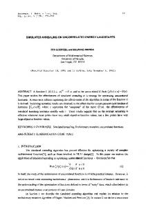
4. Simulation of hurricane and tropical storm occurrences Of real interest to oceanographers and atmospheric scientists is the yearly number of hurricanes in the Gulf of Mexico and Atlantic coast of the United States; also important, although less critical, is the frequency of tropical storms. Available data used in this study are for years 1886 to 1996. Data were obtained from the Hurricane Database (HURDAT) developed by the National Oceanic and Atmospheric Administration’s National Hurricane Center (NHC). The simplest way to simulate data is to assume independent occurrences from a standard parametric distribution. Both hurricanes and tropical storms form time series, however, suggesting the need to check for trend and autocorrelation. Simple autocorrelation functions of observations (not shown) reveal nothing remarkable in either series, but some degree of time dependence is suggested by the semivariograms. (Independent data would produce horizontal semivariograms.) The semivariogram for hurricanes is shown in Fig. 2; that for tropical storms is very similar and is omitted. Data are consistent with a constant mean process influenced by multiple sources of variation, most of which are independent but some of which are dependent, as described in section 3. Data are also consistent with an independent process model with either a linear trend or a sinusoidal mean function of period around 100 yr, peaking in the late 1960s (exact estimates depending on which series is analyzed). Indeed, with these relatively short historical series, excluding exterior information, one cannot determine whether patterns in the semivariogram truly represent correlations or else some form of cycle or trend. The point is not that any of these time series models are correct but that multiple representations may be possible for the same data, and simulations will reflect one’s choice of model. For illustration,

1 NOVEMBER 2005

4399

LOKUPITIYA ET AL.

Pr共X ⫽ x|␭兲 ⫽

␭xe⫺␭ . x!

This probability law is used to model the number of future hurricanes. Assuming there are n years in the historical record and letting xj be the number of storms that occurred in year j ( j ⫽ 1, 2, . . . , n), the parameter of the Poisson distribution ␭ is estimated by the maximum likelihood estimate n

兺x

␭ˆ ⫽ x ⫽

j

j⫽1

FIG. 2. Semivariograms of the observed (open circles) and simulated (plus signs) hurricanes.

we show in section 4b how one can use simulated annealing to capture patterns in the empirical semivariograms assuming constant mean and possible correlation, recognizing that other representations are also defensible with the data at hand. Although the storm series are not completely consistent with the assumption of independent identically distributed data, time patterns are subtle enough that even this representation would perhaps be adequate for many purposes. Regarding distributional form, hurricane occurrences are consistent with either a Poisson or a negative binomial probability model, making annealing perhaps unnecessary. Simulation using parametric modeling for hurricanes is briefly reviewed in section 4a. For tropical storms, data match well with neither the Poisson nor the negative binomial model, and a nonparameteric approach based on sample moments is recommended, with or without modeling of time patterning.

a. Parametric approaches for hurricane simulation Two parametric approaches for simulation of yearly occurrences of hurricanes are commonly used by hurricane modelers (Chen et al. 2004).

POISSON

n.

This Poisson model has two limitations. First, it assumes a constant mean number of occurrences for each year. It may be possible to improve on this simple representation by using a nonhomogeneous Poisson process, perhaps with a sinusoidal mean function as described above, but functional specifications of this type are open to criticism because of the relatively short historical series. Second, the variance of the Poisson distribution is fixed by its mean. The negative binomial distribution is frequently used to resolve this limitation. The negative binomial probability law is given by the formula Pr共X ⫽ x兲 ⫽

⌫共x ⫹ k兲 pk共1 ⫺ p兲x, ⌫共x ⫹ 1兲⌫共k兲

where k and p are parameters of the distribution. The method of moment estimates of the parameters are given by kˆ ⫽ x2/(s2 ⫺ x) and pˆ ⫽ x/s2, where n

s2 ⫽

兺x

2 j

j⫽1

冒

⫺ nx2 n.

More computationally intensive maximum likelihood estimates are generally superior (Johnson et al. 1993), but in the present applications likelihood and momentbased estimates were found to be nearly identical.

b. Nonparametric simulation of hurricanes and tropical storms We found first through fourth sample moments and sample semivariograms for the historical series. Sample semivariograms were obtained using the classical estimator

PROCESS

Each storm is considered as a point event in time, occurring independently. If ␭ is a measure of the historically based number of events per year, then for x ⫽ 0, 1, 2, . . . the probability Pr(X ⫽ x|␭) defines the probability of having x events per year, which is given by the Poisson probability formula

冒

␥ˆ 共␶兲 ⫽

兺

1 共X共ti兲 ⫺ X共tj兲兲2, ␶ ⫽ 1, 2, . . . , 2|N共␶兲| N共␶兲

where N(␶) ⫽ {(ti, tj): |ti – tj| ⫽ ␶; i, j ⫽ 1, 2, . . . , n}.Here |N(␶)| is the number of distinct pairs in N(␶) (Cressie 1993). This estimator is based on the method of moments and results directly from the formula derived in

4400

JOURNAL OF CLIMATE

section 3 under the constant mean assumption. To simulate a series of yearly occurrences that has the same correlation structure and the same distributional properties as the original series, we proceed as follows. A sample from a Poisson distribution gives a reasonable starting point, both for hurricanes and for tropical storms. In a more pathological example, an independent bootstrap sample could be used as a starting point. Here the initial configuration is taken as a series of independent values generated from the Poisson distribution with mean equal to the mean of the historical (original) series. Each new configuration is chosen by randomly selecting two values of the series, and then by increasing one value by some quantity and decreasing the other by the same quantity so that the mean of the series does not change. The semivariogram and moments are estimated for each configuration and are compared to the semivariogram and moments of the original series. We choose to impose agreement with first (mean), third (skewness), and fourth (kurtosis) sample moment properties of the original series. (Second moments are included in the semivariogram.) Sample skewness and kurtosis are included in the objective function to predict the extreme tails of the distribution. The mean, skewness, and kurtosis of the original hurricane series are 4.99, 0.58, and 3.07, respectively, and for the tropical storms they are 8.57, 0.55, and 3.72. The formal objective function used is obj共X兲 ⫽ w1

兺 ␶

关␥ˆ H共␶兲 ⫺ ␥ˆ S共␶兲兴2

2 ⫹ w2关meanH ⫺ meanS2 兴2 2Ⲑ3 ⫹ w3关skewnessH ⫺ skewnessS2Ⲑ3兴2 1Ⲑ2 ⫹ w4关kurtosisH ⫺ kurtosisS1Ⲑ2兴2,

where wi; i ⫽1, . . . , 4 are user-defined weights, ␥ˆ (␶) is the estimated semivariogram, X is a given configuration, and H and S represent the historical and simulated quantities, respectively. Exponents are chosen to remove scale effects of different moments. In the present example, each weight was set to one, but details of an objective function may be selected on a case-by-case basis. A more elaborate but possibly desirable alternative to equal weights would be to match weights to inverse variances of each component of the objective function. Obtaining estimates of moment variances would probably be best done using bootstrapping, and we maintain simplicity by using equal weights. We note that all components in the objective function are small in our example and hypothesize that the quality of simulation is fairly robust to the choice of weights.

VOLUME 18

Minimizing the objective function is equivalent to finding a series with the same mean and nearly the same covariance structure and third and fourth central moment properties as the original data. Steps of the procedure are as follows: • Step 0 (Initialize): Generate n independent random

numbers from a Poisson distribution with the observed mean (␭ ⫽ 4.99 for the hurricane series, ␭ ⫽ 8.57 for the tropical storm series). Write the initial data vector as X0 ⫽ (x01, x02, . . . , x0n). Compute the objective function for this initial configuration, obj(X0). Set Nover, the maximum allowable number of iterations at a given temperature, and Nlimit, the maximum allowable number of successful reconfigurations. Set the initial temperature T ⫽ T0, (see section 2), define the current optimal series to be Xopt ⫽ X0, and set Nsucc → 0; j → 0, i → 0. • Step 1 (Alter the configuration): Select two positions from Xi at random [say x(t1) and x(t2)]. Increase one x(t1) and decrease other x(t2) by df. We use df ⫽ 1, but this quantity could be random or fixed at some other value, depending on the application. Name the new configuration X⬘. Increment j by one ( j → j ⫹ 1). • Step 2 (Decision rule): Compute obj(X⬘). If obj(X⬘) ⬍ obj(X i ), then accept the new configuration. If [obj(X⬘) ⬎ obj(Xi)], then accept the alteration with probability p: p ⫽ exp

冉

冊

obj共Xi兲 ⫺ obj共Xⴕ兲 . T

In practice, a pseudorandom number p⬘ is generated from the uniform [0, 1] distribution and is compared with p. If p⬘ ⬍ p, the new configuration is accepted, and otherwise it is rejected. In the case of acceptance, set i → i ⫹ 1, Xi ⫽ X⬘, obj (Xi) ⫽ obj(X⬘), and Nsucc → Nsucc ⫹ 1. • Step 3 (Equilibrium criterion): Equilibrium is decided according to j ⱖ Nover or Nsucc ⱖ Nlimit, whichever comes first. If the equilibrium criterion is satisfied, then return to step 1. Otherwise, reduce the temperature by 10%. Set Xopt ⫽ Xi, and obj(Xopt) ⫽ obj (Xi). • Step 4 (Termination criterion): If obj(Xopt) is very small, then stop the search. Otherwise, set i → i ⫹ 1, j → 0, and Nsucc → 0. Set Xi ⫽ Xopt and obj (Xi) ⫽ obj(Xopt). Return to step 1. We used simulated annealing to simulate several series of hurricane and tropical storm occurrences with the same length as the historical series (111 years). Because the performance of simulated annealing is very similar for hurricane data and for tropical storms in

1 NOVEMBER 2005

LOKUPITIYA ET AL.

4401

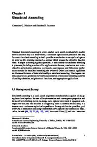
FIG. 3. Distributional properties of observed and simulated series of hurricanes: histograms of (a) observed distribution and (b) simulated series of same length as historical data hurricanes; (c) Q–Q plot of historical vs simulated hurricanes.

terms of capturing historical data properties, we only show results for hurricanes. Comparisons between historical data and a representative simulation are shown in Figs. 2–4: semivariograms are shown in Fig. 2, distributional patterns are compared using histograms and Q–Q plots in Fig. 3, and time series plots are compared in Fig. 4. In each case, agreement is good. Note that exact agreement of histograms and time series plots would in general be unrealistic but that Q–Q plots and semivariograms should match fairly well. For other simulations (not shown) variation in details of the histograms and time series plots exists, but average properties of cell frequencies agree well with historical data. Using the form of simulated annealing described above, the observed agreement between semivariograms is perhaps stronger than needed. It is also apparent from the time series plot that we replicate correlation but not the overall wave form observed in the historical data. When assessing risk for natural disasters like hurri-

canes, one must pay special attention to the extreme events that may occur in future years. The series simulated with the annealing algorithm tends to mimic the historically observed thick tails (0 and 12 occurrences for hurricanes, 1 and 21 occurrences for tropical storms). Assuming independent Poisson data, simulations also capture historical extreme cases of hurricanes adequately (about 45% of the time). Simulated annealing does capture extremes more consistently, probably because agreement is forced at the level of fourth moments, but it is possible to make simulations too similar to the historical data, and users are cautioned to select objective functions that are consistent with their needs. Conservative risk assessment may demand inclusion of plausible extremes, but other applications may favor objective functions that allow greater latitude in simulated series. We also simulated a hurricane series of 1000 years using our procedure. A histogram of this simulated se-

4402

JOURNAL OF CLIMATE

VOLUME 18

FIG. 4. Time series plots of (a) the observed hurricane series and (b) a representative simulated hurricane series of the same length.

ries indicates four extreme cases (two years with 13 hurricanes and single years with 14 and 15 hurricanes), which do not exist in the historical series but may occur in future years (see Fig. 5). More extreme values are expected in a longer series, and the simulated series reflects properties of the original series well. The number of zero occurrences was simulated to be 19, an extreme on the low end, consistent with the historical record with 2 of 111 zero occurrences.

Multiple simulations, although time consuming, could be used to show the range of expected variation in future years, assuming current physical processes continue. Success of the method for predicting plausible future hurricane numbers of course depends upon the future continuation of patterns in the last 111 years. Deviations from these patterns, whether reflections of longer natural cycles or of something such as global warming, could certainly occur.

5. Conclusions

FIG. 5. Histogram of simulated series of length 1000 years.

We have adapted simulated annealing to the problem of simulating future event occurrences such as hurricanes and tropical storms and present results. The key idea is the specification of an objective function that rewards fidelity both to marginal distributional properties and internal correlations. The method simulates a series of event occurrences similar to the given historical series without assuming a parametric form for the underlying distribution. The method was illustrated using the HURDAT database, which consists of storm

1 NOVEMBER 2005

LOKUPITIYA ET AL.

occurrences from year 1886 to 1996. The method consistently captures the extreme events, which are possible in future years. Tropical storms may be less important than hurricanes, but the tropical storm series demonstrates potential gains from annealing more dramatically. In this case, the storm counts do not follow any known distribution, yet our technique, starting from an independent Poisson “seed distribution,” successfully simulated a series that follows the properties of the historical record. The main difficulty with the method is computing cost. To simulate a series of size 1000 with the given objective function, the procedure took about 5 minutes with a MATLAB implementation on a 700-Mhz AMD processor. Substantially superior computing facilities are now common, but studies requiring a large number of simulated series, even with newer machines with high clock speed, will demand a significant commitment of computer time. Simulated annealing provides a useful if computationally intensive tool for simulating data in meteorology and climate modeling when data have complex or poorly defined distributional properties. Acknowledgments. The authors wish to thank the anonymous reviewers and the editor, Dr. David B. Stephenson, for their valuable and constructive suggestions. REFERENCES Barth, N., and C. Wunsch, 1990: Oceanographic experiment design by simulated annealing. J. Phys. Oceanogr., 20, 1249– 1263. Bennett, A. F., and B. S. Chua, 1994: Open-ocean modeling as an inverse problem: The primitive equations. Mon. Wea. Rev., 122, 1326–1336. Chen, S.-C., and Coauthors, 2003: A three-tier system architecture design and development for hurricane occurrence simulation. Proc. IEEE Int. Conf. on Information Technology: Research and Education (ITRE 2003), Newark, NJ, IEEE, 113–117. ——, and Coauthors, 2004: A web-based distributed system for

4403

hurricane occurrence projection. Software Pract. Exper., 34, 549–571. Cressie, N. A. C., 1993: Statistics for Spatial Data. Wiley, 900 pp. Deutsch, C. U., 1996: Constrained smoothing of histograms and scatterplots with simulated annealing. Technometrics, 38, 266–274. Elsner, J. B., and S. C. Schmertmann, 1993: Improving extendedrange seasonal predictions of intense Atlantic hurricane activity. Wea. Forecasting, 8, 345–351. ——, and B. H. Bossak, 2001: Bayesian analysis of U.S. hurricane climate. J. Climate, 14, 4341–4350. ——, and T. H. Jagger, 2004: A hierarchical Bayesian approach to seasonal hurricane modeling. J. Climate, 17, 2813–2827. Goovaerts, P., 1997: Geostatistics for Natural Resources Evaluation. Oxford University Press, 483 pp. Gray, W. M., C. W. Landsea, P. W. Mielke Jr., and K. J. Berry, 1992: Predicting Atlantic seasonal hurricane activity 6–11 months in advance. Wea. Forecasting, 7, 440–455. Hart, J. D., 1984: Efficiency of a Kernel density estimator under an auto regressive dependence model. J. Amer. Stat. Assoc., 79, 110–118. Johnson, N. L., S. Kotz, and A. W. Kemp, 1993: Univariate Discrete Distributions. Wiley, 565 pp. Krüger, J., 1993: Simulated annealing: A tool for data assimilation into an almost steady model state. J. Phys. Oceanogr., 23, 679–688. Lakhan, V. C., 1981: Generating autocorrelated pseudorandom numbers with specific distributions. J. Stat. Comput. Simul., 12, 303–309. Liu, M. C., and R. Taylor, 1990: Simulations and computations of nonparametric density estimates for the deconvolution problem. J. Stat. Comput. Simul., 35, 145–167. Metropolis, N., M. Rosenbluth, E. Teller, and A. Teller, 1953: Equation of state calculations by fast computing machines. J. Chem. Phys., 21, 1087–1092. Pathmathevan, M., T. Koike, and X. Li, 2003: A new satellitebased data assimilation algorithm to determine spatial and temporal variations of soil moisture and temperature profiles. J. Meteor. Soc. Japan, 81, 1111–1135. Polge, R. J., E. M. Holliday, and B. K. Bhagavan, 1973: Generation of a pseudo-random set with desired correlation and probability distribution. Simulation, 20 (5), 153–158. Press, W. H., B. P. Flannery, S. A. Teukolsky, and W. T. Vetterling, 1990: Numerical Recipes (FORTRAN Version). Cambridge University Press, 963 pp. van Laarhoven, P. J. M., and E. H. L. Aarts, 1987: Simulated Annealing: Theory and Applications. D. Reidel, 186 pp.