It is expected that current modeling and simula- tion (M&S)-driven systems
biology will be empowered by the new DEVS formalism and proposed simulation
.
Simulation Processors and Their Collaboration for DEVS Models Integrated with Universal Coupling Specification 1
Sunwoo Park1 Sean HJ Kim2 C. Anthony Hunt1,2 BioSystems Group, Dept. of Biopharmaceutical Sciences, University of California, San Francisco; 2 Joint Graduate Group in Bioengineering, University of California, Berkeley and San Francisco, 513 Parnassus Ave., San Francisco, CA 94143-0446, USA
[email protected] [email protected] [email protected]
Abstract
scribes system level biological phenomena as resulting from interactions between agents, where some agents represent biological entities and others the environment within which these entities reside [7]. An agent is commonly postulated to be an intelligent and autonomous (discrete event) system. Membrane computing, also known as P-system, provides similar capabilities for dealing with dynamic interactions covered by process algebra from a system-oriented perspective [8]. However, it does not explicitly discuss temporal aspects of the relation. It is desirable to merge the advantages of above approaches to efficiently describe and explore complex dynamic interactions of the type that occur between and inside biological systems. We have developed an advanced DEVS modeling formalism to describe adaptive spatiotemporal interactions of biological systems and the phenomena they produce [9]. The formalism has been applied to a set of biology problems including DNA formation and synthesis. It demonstrated the power and effectiveness of the new formalism in describing dynamic spatiotemporal interactions and the temporal dynamics that occur between and within biological systems. In this paper, we present a set of simulation processors and describe their temporal collaboration to execute models described by the new modeling formalism. Proposed simulation processors extend an existing parallel DEVS abstract simulator and coordinators by integrating the universal interaction mechanism [9][10]. The universal interaction specification and revised DEVS model specifications will be briefly described before simulation processors are presented.
We present a set of simulation processors and describe their temporal collaboration in support of the execution of models specified by an advanced Discrete Event Systems Specification (DEVS) formalism. Our formalism improves the existing parallel DEVS formalism by adopting the universal coupling mechanism. The mechanism enables coupled models to create, permute, and delete their couplings in a proactive or reactive manner. Each coupled model is a decomposable, constructive, multi-scale, discrete-event system that contains at least one component. Proposed simulation processors will allow exploration of spatiotemporal spaces generated from specified models. A simulation protocol is realized as a sequence of welldefined temporal interactions between those processors. It is expected that current modeling and simulation (M&S)-driven systems biology will be empowered by the new DEVS formalism and proposed simulation processors.
1
Introduction
Many complex biological phenomena result from dynamic spatiotemporal interactions between components and subsystems. To cope with the dynamic nature of the interactions, several computational methods have been applied. Process algebra describes an interaction between systems as a set of communication link and its dynamic permutation [1][2][3]. It focuses mainly on relationships between systems rather than on their internal temporal dynamics. Meanwhile, discrete event systems and discrete-event driven M&S focus on the temporal dynamics of systems [4][5][6]. They describe an interaction by message (or event) exchange or propagation links. The message is consumed or produced by a system as the result of a reactive response to incoming messages or its proactive dynamic state transitions. Specifically, agent-based M&S de-
2
Universal coupling
A coupling is a directional influence from one entity to another. The influencer and influencee are commonly described as a pair: a model and its property (e.g., communication I/O port). It is classified into three categories: static, dynamic, and adaptive.
151
ar : (mi , pi , mj , pj , ∗, ∗, ξ, ρ, l, ψ, ϕ). The binding Ci,j function ϕ : C ar → C d resolves the meta candidate d∗ ar , ψ, ϕ) is its endomor: (Ci,j when ψ is satisfied. Ci,j phic representation.
A static coupling consists of one influencer (mi , pi ) and one influencee (mj , pj ). It represents a causal relation from the influencer to the influs encee. The coupling is specified by a 4-tuple Ci,j : (mi , pi , mj , pj ) where mi , mj ∈ M , pi , pj ∈ P , M is a set of models, and P is a set of properties.
a
u s d A universal coupling Ci,j : Ci,j ⊕ Ci,j ⊕ Ci,∗p ⊕ a ar is the composition of all couplings introC∗,jp ⊕ Ci,j duced above. See [4] and [9] for more details on coupling mechanisms.
A dynamic coupling is an extension of the static coupling that enables its dynamic permutation. Dynamic permutation includes the change of influencer or influecee, construction of a new static or dynamic coupling, and destruction of an existing dyd namic coupling. It is specified by a 9-tuple Ci,j : (mi , pi , mj , pj , mk , pk , ξ, ρ, l) where mi , mj , mk ∈ M , pi , pj , pk ∈ P , ξ is a coupling constraint, ρ : C d → C d is a coupling permutation function, and l ∈ Z + is a lifespan variable. It can be alternatively specified by an d s endomorphic 5-tuple Ci,j : (Ci,j , mk , pk , ξ, ρ, l) where s Ci,j is a static coupling, mk , pk , ξ, ρ, and l are as same as above. (mk , pk ) is the candidate that will be promoted to a new influencer or influencee after dynamic permutation. ξ specifies when the permutation occurs. Satisfying ξ triggers ρ. ρ provides details on how the coupling is changed. The dynamic coupling is valid only when l > 0. l can be increased or decreased after execution of ρ. An important property of the coupling is its capability to construct, permute, and evolve coupling networks from an existing coupling or coupling network. By tracking changes in network topology, we can trace dynamic coupling permutation between models during their lifetime.
3
DEVS coupled model with universal coupling
Our new DEVS coupled model strengthens the existing coupling specification of Parallel DEVS (PDEVS) by replacing it with the universal coupling specification [4][9][10]. For the congruent integration of the universal coupling specification with the DEVS formalism, we use causal relation forms instead of tuples. Specifically, (mi , pi ) → mk ,pk ,ξ,ρ,l
s (mj , pj ) for Ci,j , (mi , pi ) −−−−−−−→ (mj , pj ) for d Ci,j , (m∗ , p∗ )
(mi , pi )
mk ,pk ,ξ,φ,ρ,l,ψ,ϕ
a
−−−−−−−−−−−→ (mj , pj ) for C∗,jp ,
mk ,pk ,ξ,φ,ρ,l,ψ,ϕ
−−−−−−−−−−−→
a
(m∗ , p∗ ) for Ci,∗p , and
m∗ ,p∗ ,ξ,φ,ρ,l,ψ,ϕ
ar (mi , pi ) −−−−−−−−−−−→ (mj , pj ) for Ci,j .
The DEVS coupled model with the universal coupling N is hX, Y, D, {Md }, {Id }, {Zd,i }i. X is a set of inputs. Y is a set of outputs. D is a set of components. For each d ∈ D, Md is a DEVS model, which is either atomic or coupled. For each d ∈ D ∪ {self }, Id is the set of influencees of d. self is a reserved reference of N itself. For each i ∈ Id , Zd,i is a function, d-to-i output p s d r s translation with Zd,i ∈ (Zd,i ∪ Zd,i ∪ Zd,i ∪ Zd,i ). Zd,i is the static translation function with (i) Zd,i : X − → Xi , if d=self ; (ii) Zd,i : Yd − → Y , if i=self ; and (iii) Zd,i : d Yd − → Xi , if d 6= self ∧ i 6= self . Zd,i is the dynamic
An adaptive coupling is an extension of the dynamic coupling that permits meta entities in the coupling specification. The entities are not precisely described in an initial specification. However, they are adaptively resolved and bound to concrete entities at later times. The coupling is mainly used to adaptively create a dynamic coupling in a proactive or reactive maner. It divides into two adaptive couplings proactive and reactive. A proactive coupling is an extension of the dynamic coupling that contains a meta influencee or influencer (∗, ∗), a binding constraint ψ, and a binding function ϕ : C ap → C d . (∗, ∗) is resolved and bound by ϕ when ψ is satisfied. ϕ creates a dynamic coupling. The coupling is represented a by a 11-tuple Ci,∗p : (mi , pi , ∗, ∗, mk , pk , ξ, ρ, l, ψ, ϕ) or ap C∗,j : (m∗ , p∗ , mj , pj , mk , pk , ξ, ρ, l, ψ, ϕ), respectively, depending on the existence of the meta influencer or influencee. It is alternatively simplified to an endora a d d morphic 3-tuple - Ci,∗p : (Ci,∗ , ψ, ϕ) or C∗,jp : (C∗,j , ψ, ϕ). A reactive coupling is an adaptive coupling that contains a meta candidate. Unlike the proactive coupling, the influencer and influencee are “clearly” presented but the candidate (mk , pk ) is not precisely defined in the coupling. The coupling is denoted as
Xk ,ξ,ρ,l
translation function with (i) Zd,i : X −−−−−→ Xi , Yk ,ξ,ρ,l
if d=self ; (ii) Zd,i : Yd −−−−−→ Y , if i=self ; and Xk ,ξ,ρ,l
(iii) Zd,i : Yd −−−−−→ Xi , if d 6= self ∧ i 6= self . p Zd,i is the proactive translation function with (i) Zd,i : Xk ,ξ,ρ,l,ψ,ϕ
Yk ,ξ,ρ,l,ψ,ϕ
X −−−−−−−−→ X∗ , if d=self ; (ii) Zd,i : Y∗ −−−−−−−→ Xk ,ξ,ρ,l,ψ,ϕ
Y , if i=self ; and (iii) Zd,i : Y∗ −−−−−−−−→ Xi or Xk ,ξ,ρ,l,ψ,ϕ
Yd −−−−−−−−→ X∗ , if d 6= self ∧ i 6= self , where r ∗ ∈ D is an unspecified component. Zd,i is the reactive X∗ ,ξ,ρ,l,ψ,ϕ
translation function with (i) Zd,i : X −−−−−−−−→ Xi , Y∗ ,ξ,ρ,l,ψ,ϕ
if d=self ; (ii) Zd,i : Yd −−−−−−−→ Y , if i=self ; and X∗ ,ξ,ρ,l,ψ,ϕ
(iii) Zd,i : Yd −−−−−−−−→ Xi , if d 6= self ∧ i 6= self .
152
4
Simulation protocol
the amount of σmin , which is min{σd | d ∈ D} where σd = τ (sd ) − ed . sd , ed , τ (sd ), and σd are s, e, τ (s), and σ(s) of Md ∈ M , respectively. IM M is the set of imminent components that produce outputs, {d | σd = τ (sd ) ∧ λbd (sd ) 6= φ}, at time tL + σmin . λbd (sd ) is the bag of output messages produced by Md . IN F is the set of components influenced by d ∈ IM M , {i | i ∈ Id , d ∈ IM M ∧ xbi 6= φ} where xbi = {Zd,i (λbd (sd )) | d ∈ IM M ∩ Id }. It is equivalent to {d | d ∈ D ∧ xbd 6= φ} in the algorithm we present here because λbd (sd ) produced by each d ∈ IM M is translated to {xbi }i∈D through Zd,i (λbd (sd )) based on Id before IN F is computed. Dynamic or adaptive permutation is managed when the coordinator receives the message (!, t) from its parent coordinator. A collection of Algorithm 2 and 3 represents a coordinator that refines and extends the P-DEVS coordinator with the integration of the universal coupling specification.
For simulation time management, we use tL , t, tN , e, σ to represent the time the last event occurs, the current simulation time, the time the next event will occur, the elapsed time since tL , and the time left until tN , respectively. Specifically, e = t − tL , σ = tN − t = tN − (tL + e), and tN = tL + τ (s) = t + σ where tL ≤ t ≤ tN .
Algorithm 2 Coordinator for a coupled model: Part I
Figure 1: DEVS simulation time
1: 2: 3: 4: 5: 6: 7: 8: 9: 10: 11: 12: 13: 14: 15: 16: 17: 18: 19: 20: 21: 22: 23: 24: 25: 26: 27: 28: 29: 30: 31: 32: 33: 34: 35: 36: 37: 38: 39: 40: 41:
There exist three different simulation processors - root coordinator, coordinator, and simulator. A root coordinator controls the top-most coordinator. Each coordinator controls its components by exchanging simulation control messages with both its parent coordinator and child components. Each simulator executes its associated atomic model whenever it receives a simulation control message from its parent coordinator. Algorithm 1 presents an atomic simulator that refines the original P-DEVS abstract simulator. Algorithm 1 Simulator for an atomic model 1: 2: 3: 4: 5: 6: 7: 8: 9: 10: 11: 12: 13: 14: 15: 16: 17: 18: 19: 20: 21: 22: 23: 24: 25:
tL := e := 0; tN := τ (s); xb = φ when (%, t) message arrives from parent send (%, τ (s) - (t - tL )) to parent end when when (@, t) message arrives from parent send (y, ((t = tN ) ? λ(s) : φ), t) to parent end when when (x, xbd , t) message arrives from parent xb := xb ⊕ xbd send (done, t) to parent end when when (∗, t) message arrives from parent if t < tL ∨ t > tN then timing synchronization error else e := t - tL if tL ≤ t ≤ tN then s := (xb 6= φ) ? δext (s, e, xb ) : s else if t = tN then s := (xb = φ) ? δint (s) : δconf (s, e, xb ) else raise error end if tL := t; tN := tL + τ (s); xb := φ send (done, tN ) to parent end if end when
A coordinator advances the simulation time by
153
tL := tN := e := 0; sync := φ when (#, t) message arrives from parent sync := D for each d ∈ D do send (%, t) to child d end for end when when (%, t) message arrives from child d σd := t; sync := sync\d if |sync| = 0 then tN := tL + min{σd } send (done, tN ) to parent end if end when when (@, t) message arrives from parent IM M := IN F := φ; sync := D for each d ∈ D do xbd := φ send (@, t) to child d end for end when when (y, y b , t) message arrives from child d sync := sync\d if y b 6= φ then IM M := IM M ⊕ d for each i ∈ Id \self do xbi := xbi ⊕ zd,i (y b ) end for b b if self ∈ Id then yself := yself ⊕ zd,self (y b ) end if end if if |sync| = 0 then b send (y, yself , t) to parent b yself := φ end if end when when (x, xb , t) message is received from parent for each i ∈ Iself ∧ xb 6= φ do xbi := xbi ⊕ zself,i (xb ) end for for each d ∈ D ∧ xbd 6= φ do IN F := IN F ⊕ d end for sync := IN F for each d ∈ IN F do send (x, xbd , t) to child d end for end when
Algorithm 3 Coordinator for a coupled model: Part II 42: 43: 44: 45: 46: 47: 48: 49: 50: 51: 52: 53: 54: 55: 56: 57: 58: 59: 60: 61: 62: 63: 64: 65:
topology. Proposed simulation processors enable exploration of spatiotemporal spaces generated by dynamic construction and permutation of interactions between biological system components. Our expectation is that these processors and the revised formalism will facilitate progress in how the hierarchical, multiscale mechanistic details of biological systems can be modeled, coupled, and simulated.
when (!, t) message is received from parent for each z in Z do a a if z ∈ (Ia p ⊕ Iaar ⊕ Ie p ⊕ Iear ) then if z.ψ is true then execute z.ϕ end if else if z ∈ (Iad ⊕ Ied ) then if z.ξ is true then execute z.ρ end if end if end for end when when (∗, t) message is received from parent e := t - tL if tL ≤ t ≤ tN then sync := IM M ⊕ IN F for each d ∈ IM M ⊕ IN F do send (∗, t) to child d end for end for else raise an error end if tL := t end when when (done, t) message arrives from child d sync := sync\d if |sync| = 0 then send (done, t) to parent end if end when
Acknowledgements This research was funded in part by CDH Research Foundation, Postdoctoral Fellowship provided to SP by CDH R.F., and Graduate Fellowship to SHJK from IFER. We thank Prof. Bernard P. Zeigler and other members of the BioSystems Group for helpful discussion and commentary.
References [1] R. Miller, Communicating and mobile systems: the π-calculus. Cambridge University Press, 1999.
The root coordinator initiates the whole simulation cycle by sending the (#, tN ) message to the top-most coordinator and terminates it if tN is ∞.
[2] C. Priami, “Stochastic π-calculus,” The Computer Journal, vol. 38, no. 7, pp. 578–589, 1995.
Algorithm 4 Root coordinator
[3] A. Regev, E. M. Panina, W. Silverman, L. Cardelli, and E. Shapiro, “Bioambients: an abstraction for biological compartments,” Theoretical Computer Science, vol. 325, no. 1, pp. 141– 167, 2004.
1: tN := 0 2: while tN 6= ∞ do 3: send (#, tN ) to the top coordinator 4: wait for (done, tN ) from the top coordinator 5: send (@, tN ) to the top coordinator 6: wait for (y, y b , tN ) from the top coordinator 7: send (x, xb , tN ) to the top coordinator 8: wait for (done, tN ) from the top coordinator 9: send (!, tN ) to the top coordinator 10: wait for (done, tN ) from the top coordinator 11: send (∗, tN ) to the top coordinator 12: wait for (done, tN ) from the top coordinator 13: end while
[4] B. P. Zeigler, T. G. Kim, and H. Praehofer, Theory of Modeling and Simulation, ser. 2nd edition. Academic Press, 2000. [5] J. Banks, I. John S. Carson, and B. L. Nelson, Discrete-Event System Simulation. PrenticeHall, 1996. [6] R. Y. Rubinstein and B. Melamed, Modern Simulation and Modeling. Willey, 1998.
5
Conclusion
[7] P. Davidsson, B. Loga, and K. Takadama, Eds., Multi-Agent and Multi-Agent-Based Simulation: Joint Workshop MABS 2004, ser. Lecture Notes in Computer Science, vol. 3415. Springer, 2005.
We present a set of three simulation processors to execute and control models specified using the advanced DEVS modeling formalism. The formalism defines coupling relations between components of a coupled model with the universal coupling specification. The formalism enables dynamic creation, permutation, and removal of couplings in a proactive or reactive manner. With this feature, the coupling networks between components in a coupled model can be evolved during simulation. The evolution can be traced by tracking changes in the coupling network
[8] G. Paun, “Computing with membranes,” Journal of Computer and System Sciences, vol. 61, pp. 108–143, 2000. [9] S. Park and C. A. Hunt, “Coupling permutation and model migration based on dynamic and adaptive coupling mechanisms,” in The Proceedings of the 2006 DEVS Symposium, 2006.
154
[10] A. C. Chow and B. P. Zeigler, “Parallel DEVS : A parallel, hierarchical, modular modeling formalism,” in Proceedings of the 1994 Winter Simulation Conference, 1994.
155