In this paper an alternative approach to LMN and gain scheduling, refered to as simultaneous D ... steering angle) and the output y (physically, offset y) yields. 3.
Simultaneous D-stabilisation robust controller design for autonomous vehicle steering Yongji Wang, Michael Schinkel, Tilmann Schmitt-Hartmann and Ken J. Hunt Centre for Systems and Control, Dept. of Mechanical Engineering, James Watt Building, University of Glasgow, Glasgow, G12 8QQ, Scotland, U.K. Tel: (+44) 141 330 4370 Fax: (+44) 141 330 4343 email:{ywang, k.hunt}@mech.gla.ac.uk
Abstract This paper presents a new robust controller design method for autonomous vehicle steering, satisfying the non-switching simultaneous D-stability requirement. The non-linearity of the vehicle introduced by variable speed and mass of the vehicle is characterised by the linearised time-invariant models at various operating points which cover the full range of the operating regimes. In this way parameter variations caused by varying speed and mass from road slope and load changes can be taken into account. The simultaneous D-stabilisation robust controller design method permits the designer to specify a set of desired D stable regions, joint or disjoint, in the complex root plane, and then a numerical algorithm is used to find the design controller parameters such that all the roots of the closed-loop systems resulting from the linearised plant models are within the specified regions. This general D-stable design method allows for the simultaneous consideration of the stability and transient performance. Simulation results are provided to illustrate its merit. Key words: Automotive control, autonomous vehicle, autonomous robot, non-linear control, robust control, simultaneous stabilisation, non-linear models, gain scheduling.
1. Introduction Urban and suburban freeway congestion has been increasing rapidly in recent years, particularly in the largest and fastest-growing metropolitan areas. Research indicates that this trend will be continuing and indeed becoming even more acute in the coming years. More recently, some researchers have been applying advanced electronics technologies to provide drivers with real-time information about congestion, as well as navigation and route guidance information, see [32] and the references therein. It is estimated that all of these measures together may be able to improve the utilisation of existing road facilities by 15 or 20 percent, but that is not enough to meet present and anticipated future needs. In order to provide the more substantial increases in the throughput that are needed, one solution is the development of Intelligent Transportation Systems (ITS). This would mean that it is necessary to automate the control of the vehicles. At the very least, the steering, acceleration and braking of the vehicles would be automatically controlled, without the direct intervention of a human driver. To this end, a robust controller must be designed to deal with the uncertainties resulting from the changes of road condition, of the mass and of the varying vehicle speed and other factors. For controller design a vehicle dynamic model is needed. The lateral vehicle dynamics in response to applied steering inputs are very complex [11-17,1]. It includes a number of uncertain parameters. A detailed description of this is given in [22], and simplified models suitable for robust controller synthesis are described by [1,11,15]. The large-signal non-linear dynamic model is so complex that it must be simplified for the purpose of controller design. As shown previously [1,11-17], controller design based on a small-signal deviation model still presents something of a challenge as it is a linear system with time–varying parameters. The parameters of the linear model depend on a number of physical constants such as vehicle mass and speed. The controller designed has to work over the full range of vehicle speed and mass. A number of papers have been devoted to the investigation of robust controller design for autonomous vehicle control. Ackermann [1] proposes a control structure having two parts; a decoupling
1
compensator, and a variable gain part in which the controller gains depend continuously on the measured speed. With this structure, only one uncertain parameter is considered (mass) and a robust control design is performed to ensure a desired degree of stability and performance in the face of assumed mass variations. Based on the similar idea, a controller is redesigned recently by Jia [15]. An alternative control approach is taken by Mecklnburgh et al. [21] who developed a neural-networkbased controller by optimising a non-linear control function. Recently, based on the representation of non-linear plants by local model networks (LMN) [11,12,13], a non-linear control structure known as local controller network (LCN) has been proposed [11,12,13]. The structure consists of a convex combination of a number of individual controllers, each of which is valid locally in the state or input space of the plant. Gain scheduling, an attempt to apply the well-developed linear control methodology to the control of non-linear systems, has been adopted [14,17]. The idea of gain scheduling based on LMN is to select a number of operating points, which cover the range of the system operations. Then at each of these points, the designer makes a linear time-invariant approximation to the plant dynamics and designs a linear controller for each linearised plant. Between operating points, the parameters of the compensators are then interpolated, or scheduled, thus resulting in a global compensator. Gain scheduling is conceptually simple, and indeed, practically successful for a number of applications. The main problem with gain scheduling is that it has only limited theoretical guarantees of stability in nonlinear operation. It uses some loose practical guidelines such as “the scheduling variables should change slowly” and “the scheduling variables should capture the plant’s nonlinearities”. For more details on LMN, LCN and gain scheduling based on linearisation about a set of equilibrium points and off-equilibrium points, see [11-14,16-17]. In this paper an alternative approach to LMN and gain scheduling, refered to as simultaneous D stabilisation (SDS), is applied. This new robust controller design approach is first proposed in [33,34]. We still use the method of LMN to represent the time-varying plant models. However this approach tries to find a non-switching, fixed-order controller such that all the roots for the local plant models are respectively placed within a set of desired regions, referred to as D stable regions, in the complex root plane, thus reducing the need to interpolate the local controllers. It is noted that the SDS approach is different from either the traditional root locus approach in classic control, or the pole assignment and linear quadratic regulator approaches in modern control. Compared with root locus approach the advantage of the SDS approach is that it can deal with more than one unknown design parameters in controller and more than one plant models. On the other hand compared with pole assignment and linear quadratic regulator approaches, its advantage is that it does not need full states for feedback which may not be available for many practical applications. The transient performance of the closed systems is improved by changing the D-stability regions in the complex plane.
2. Lateral vehicle dynamics and simultaneous D-stabilisation problem 2.1 Lateral vehicle dynamics with time-varying parameters In this subsection a very brief outline of the lateral vehicle dynamics is given. It is based upon [1], where a simplified but nevertheless realistic version of the comprehensive model of [22] is presented. The main variables used in the model are depicted in Fig. 1.
δ
steering angle
ψ yaw angle
β υ side slip angle
y: lane offset
Fig. 1 Control of lateral vehicle position
2
r
δf
uf
e Controller
y Steering dynamics
Actuator
-
(a)
r
uf
e C(s)
y G i(s)
-
(b)
Fig. 2 Autonomous steering of a vehicle. The error e=r-y between guideline r and sensor position y is measured. For straight line as a guide line r=0. The plant dynamic model consists of two parts: the steering dynamic model and the actuator model, see Fig. 2 (a). A linearised steering dynamic model for the lateral vehicle dynamics is given by (see the appendix A in [1] y( s ) n( s) = δ f ( s) d ( s )
(1)
where d(s) and n(s) have the forms of d(s)=s 2(a0+a1s+s2), n(s)= b0+b1s+b2s2, respectively. The system output is the offset y. The control input is the steering angle δ f. The steering angle is normally established by an integrating actuator. The control signal for the system uf is therefore related to the steering angle by
δ& f = u f
(2)
Combining the two preceding transfer-functions between the input uf (physically, rate of change of steering angle) and the output y (physically, offset y) yields
c f v(e 0 + e1 s + e2 s 2 ) y (s ) = G ( s) = u f (s) ( d 0 + d 1s + d 2 s 2 ) s 3 where
(3)
e0=crlv e1=crl(lr+ls) e2=(i2+lslf)mv d0=cfcrl2+(crlr-cflf)mv2 d1=[(cr+cf )i2+(cfl2f+crl2r)]mv d2=i2m2v2
and cr(cf) is the cornering stiffness for the rear wheels(front wheels). The distances lr and lf from the centre of gravity to the rear and front axles sum up to the wheelbase l=l r+lf. ls represents the distance of the sensor mounted on the vehicle to the gravity centre. m is the normalised mass by a road adhesion factor µ, i.e. m=mreal/µ. Similarly the moment of inertia J is normalised as J=J real/µ, and i, referred to as inertial radius, is defined by the relationship of J=i 2m. v is the velocity of the vehicle. In the transfer function model (3) the following eight parameters have been used: cf,cr,m,i,v,l f,l r,l s. As the driving conditions change, those parameters also change. However these uncertain parameters are not mutually independent. For example the vehicle has a fixed wheelbase, i.e l=l r+lf=constant. Also the fact that the moment of inertia and the mass of the vehicle is not independent leads to the dependence of the inertia radius i on normalised mass m [1]. In addition the uncertainty due to the other five parameters cf,cr,l f,l r,l s can also be related to the uncertainty of m in some ways, therefore in this paper only m and v are considered as uncertain parameters. The data for a typical vehicle (city bus O 305) are shown in Table 1 and will be used later in this paper [1].
3
Table 1 Data for the city bus O 305 lf 3.67 [m]
lr 1.93 [m]
ls 6.12 [m]
cf 198000 [N/rad]
cr 470000 [N/rad]
v [3;20] [m/s]
m [9950;32000 ] [kg]
i2 10.85 [m2]
The transfer function (3) from actuator input to lateral deviation for the data given in Table 1 is G (s) =
4.803 ⋅ 1010 v 2 + 3.866 ⋅ 10 11 vs + 6.079 ⋅ 10 5 mv 2 s 2 ( 2. 690 ⋅ 1011 + 1 .663 ⋅ 10 4 mv 2 + 1.075 ⋅ 10 6 mvs + m 2v 2 s 2 ) s 3
(4)
2.2 Local operating-point-based linearised plant model It is important to note that the numerator and denominator coefficients of the plant transfer-function (4) depend on the vehicle speed v and mass m, thus resulting in a linear time-varying system. The parameters v and m determine the operating regimes. As mentioned in [11,12,13], the partioning of the parameter-space into operating regimes is selected such that each local model is reasonably accurate in the region where it will be applied between the gridded parameter points. If the variations of v and m are respectively characterised by nv and nm points associated with each operating point vi and mj, then the plant dynamics (4) may be approximately represented by nv×nm local linearised models, as shown in Fig. 3 where nv×nm =4×4. Let Gij(s) denote the ij-th local time-invariant plant model, from (4) and Table 1 we have 4.803 ⋅1010 vi + 3.866 ⋅10 11 vi s + 6.079 ⋅10 5 vi m j s 2 2
Gij ( s) =
2
( 2.690 ⋅1011 + 1.663 ⋅10 4 vi m j + 1.075 ⋅10 6 vi m j s + vi m j s 2 ) s 3 2
2
2
, i=1,2,…,nv, j=1,2,…,nm
(5)
m m4 m3 m2 m1 v v1
v2
v3
v4
Fig. 3 Operating regimes for autonomous vehicle. These regimes are characterised by vehicle velocity and mass
2.3 Description of desired D-stability regions It is well known that an important issue in the theory and practice of control system synthesis is the design of a feedback controller that places the closed-loop poles of a linear system at desired regions. In this paper we extend this idea to multiple linear plant models, which results in the simultaneous Dstabilisation problem [34,35]. We first introduce the important concept of D stability. Let D denote the interior of a region in the complex plane, ∂D denotes its boundary. For a continuous time system, if a region is located in the left half of the complex plane this region is said to be a D-stable region, and its boundary is said to be a D-stable boundary. In control system design all the closed-loop poles should be confined to a desired D-stable region or a set of disjoint desired D-stable regions. We shall say that the closed-loop system is D-stable if all the roots of its characteristic polynomial are located in the desired D-stable regions.
4
A distinguished feature that makes the approach used in this paper different is that the general D stable regions, joint or disjoint, are here expressed by inequalities, which, combining with other equality constraint representations, leads to the efficient numerical algorithms used in section 4. This feature also makes it possible to investigate controller design issues for both continuous and discrete systems in a unified way, although this paper is only devoted to continuous systems. We call an inequality of the form g(x)