Size Distribution of Multikilometer Transneptunian Objects - Caltech GPS

Petit et al.: Size Distribution of Multikilometer Transneptunian Objects

71

Size Distribution of Multikilometer Transneptunian Objects J-M. Petit Observatoire de Besançon

JJ Kavelaars Herzberg Institute of Astrophysics

B. Gladman University of British Columbia

T. Loredo Cornell University

There are two main goals in studying the size distribution of the transneptunian objects (TNOs). The first is the quest to determine the mass in the transneptunian region. The second is to understand the competition between accretion and collisional erosion. The size distribution of the largest bodies is controlled by the accretion process, while that of bodies smaller than 50–100 km in diameter is believed to result from collisional evolution. An accessible way to determine the size distribution of TNOs is to determine their luminosity function (LF) and then try to convert magnitude to size. Interpreting the survey data to determine the correct LF, with confidence region for the parameters, is a subtle problem and is only beginning to be properly understood. Converting the LF into a size distribution is very complex and involves modeling, both dynamical and of physical surface properties of the TNOs. Several papers have been published that address this question, yielding LF slope of 0.3 to 0.9, and 1 object per deg2 brighter than R magnitude 23–23.5. The exponent of the size distribution is most likely on the order of 4–5 for bodies larger than a few tens of kilometers, and the number of objects with diameter larger than 100 km is on the order of a few 104. However, this subject is still in its infancy, and much observational and modeling work needs to be done before we claim to know the size distribution of the various populations of TNOs.

1.

per belt environment (Farinella and Davis, 1996), and their size distribution is therefore directly linked to the accretion processes. Even in the denser collisional environment of the early solar system, these bodies must have been safe, as the mass depletion of the belt must have resulted from dynamical erosion rather than collisional erosion (Petit and Mousis, 2004; Morbidelli and Brown, 2004). Smaller than 50–100 km in diameter, the TNOs should have suffered strong collisional evolution, and their current size distribution is connected to their physical properties and collisional environment (Davis and Farinella, 1997).

INTRODUCTION

In this chapter, we consider another aspect of transneptunian object (TNO) discovery called the luminosity function (LF), which we then relate to the size distribution of these small bodies. Discovering TNOs goes beyond the simple fact of finding yet other small bodies in the solar system. Our ultimate goal is to understand, through the knowledge of the current small-body populations, the formation and evolution processes of our solar system, and potentially of other planetary systems. Much of the motivation for observational and cosmochemical studies of small bodies stems from the desire to use the results to constrain or otherwise illuminate the physical and chemical conditions in the early solar system, in the hope of learning more about the processes that led to the formation of our planetary system. As will be seen in the chapter by Kenyon et al., the size distribution of the TNO population holds clues to the process of giant-planet and small-body formation and the collisional evolution of the latter. Large bodies are most likely immune to collisional disruption over the age of the solar system in the current Kui-

2. HISTORICAL REVIEW The long history of asteroid observations designed to explore the asteroid main-belt size distribution in order to study collisional physics extends naturally to the Kuiper belt. Even after more than a decade of Kuiper belt exploration, the value of the fundamental property of the belt’s mass still varies in the literature. The asteroid belt’s size distribution is decently approximated by power laws over certain diameter ranges. Assuming this also holds for the 71

72

The Solar System Beyond Neptune

Kuiper belt, astronomers have tried to estimate the mass in objects of a given (observable) size, then use the slope of the apparent magnitude distribution to estimate the slope of the diameter distribution and finally estimate the Kuiper belt mass by integrating the power law from the reference point to upper and lower limits. Firm determination of a reference object size requires either resolving objects in the optical (thus directly measuring diameter) or obtaining both optical and thermal infrared observations to use thermal modeling to estimate a diameter. Only three of the largest TNOs (Pluto, Quaoar, and Eris, formerly 2003 UB313) have been resolved, all using the Hubble Space Telescope (HST) (Albrecht et al., 1994; Brown and Trujillo, 2004, 2006); the diameter estimates for Eris thus obtained are still only accurate at the 5% level. Pluto and Eris are shown to have albedos more than an order of magnitude larger than the value of 4% often used in the literature. The promising avenue of detection of the thermal IR flux from large TNOs has yielded mixed results, as several of the known large TNOs have not been detected by the Spitzer Space Telescope (see chapter by Stansberry et al.), presumably also because most TNOs have albedos far above the 4% figure. Only the most nearby (and thus warmest) large TNOs have yielded diameter estimates from their IR emission. That determining the size distribution was necessary for measuring the Kuiper Belt mass was recognized at the time of the discovery of 1992 QB1 (Jewitt and Luu, 1993). With additional discoveries, the measurement of the so-called luminosity function, or LF, has become an important goal of observational Kuiper belt surveys. The LF simply gives either the cumulative or incremental number of TNOs brighter than a given apparent magnitude; it is often given relative to a surveyed area of 1 deg2. The usual functional form used is an exponential for the cumulative LF like Σ(m) = 10α(m – m o)

(1)

with α being the slope and mo the magnitude at which one would expect to have 1 object per deg2 of sky. Conversion of the LF to a size distribution requires certain assumptions (discussed below), which can lead to a power law. But even the measurement of the apparent magnitude distribution requires careful analysis of sky surveys. Determining the slope of the apparent magnitude distribution requires a reasonable number of TNOs to be discovered in a survey of known area and known sensitivity. In order to be of any use for further modeling and/or comparison with other works, the surveys need to publish their areal coverage, the TNO magnitudes (with errors), and (very importantly) the characterization of their detection efficiency as a function of magnitude (at least; giving it as a function of other observing parameters like the rate of motion can be very useful too) for each portion of their discovery fields. Actually, the publication of the full information necessary for the reader to be able to redo the work is mandatory in a scientific publication. Otherwise, we are no longer using a scientific approach, but are merely relying on faith.

In the following we list the works that explicitly addressed the question of LF determination. We separate the surveys between those that satisfied the above requirements (Table 1) and those that did not (Table 2). In the first category, we have the work by Jewitt and Luu (1995), Irwin et al. (1995), Jewitt et al. (1998), Gladman et al. (1998, 2001), Chiang and Brown (1999), Trujillo et al. (2001a,b), Bernstein et al. (2004), Petit et al. (2006), and Fraser et al. (personal communication, 2007), whose main characteristics are summarized in Table 1. We divided them into two categories: surveys in which the objects are visible on each individual frames (wide-area surveys), and surveys in which several images were stacked together after shifting to reveal the objects (small-area deep surveys). For the sake of completeness, we also list the surveys that addressed the LF determination, but did not meet the above requirements: Jewitt et al. (1996), Luu and Jewitt (1998), Sheppard et al. (2000), Larsen et al. (2001), and Elliot et al. (2005). The first two works did not publish their efficiency function, while the last three only sparsely sampled the efficiency function on a few frames and/or did not provide the information necessary to match efficiency functions to specific sky coverage. Table 2 gives the characteristics of this second set of surveys. Other KBO surveys have been performed over the years, but were intended to simply find objects, and/or determine dynamical information, not LF, and are thus not described in this chapter. However, the most important ones, which were used as constraints in the works presented here, are Tombaugh (1961) (T61), Luu and Jewitt (1988) (LJ88), Kowal (1989) (K89), Levison and Duncan (1990) (LD90), and Cochran et al. (1995) (C95). T61 and K89 were photographic plate surveys, LJ88 and LD90 were groundbased CCD surveys, and C95 was a space-based, HST survey. 2.1.

Wide-Area Surveys of Transneptunian Objects

Large-scale surveys typically cover from several square degrees (deg2) up to a few thousand, reaching a limiting mR magnitude of 24 or brighter. The goal is to detect a large number of objects in each of a small number of CCD images taken of the same sky region at 1- to 24-h spacing. They generally use detections on single images and search for objects whose measured position changes from frame to frame at rates consistent with outer solar system targets. The relatively bright targets detected are then suitable for tracking over the several-year baseline needed to determine an orbit; however, under certain assumptions, knowledge of the orbit is not required to determine the LF. Such survey can essentially provide an estimate of the “zeropoint” (at which magnitude mo there is one object per deg2 brighter than mo) and the slope. A major potential complication of such an approach is that there are good reasons to expect that the on-sky surface density will vary with ecliptic latitude and longitude. A change in mo (to fainter magnitude) is expected as one departs from the plane of the solar system as the spatial den-


TABLE 1.

73

List of past characterized luminosity function (LF) surveys.

Abbrev.

Ω* (deg2)

N†

ηmax‡

m50§

R.A.¶ (2000)

l** (deg)

Comments

Wide-Area Surveys Jewitt and Luu (1995)

JL95

1.2

7

1.

24.8

ITZ95 JLT98

0.7 51.5

2 13

1. 0.91

23.5 22.5

Trujillo et al. (2001a)

TJL01

73

86

0.83

23.7

Trujillo et al. (2001b)

T01

164

4

0.85

21.1

Petit et al. (2006)

P06

5.97 5.88

39 26

0.90 0.90

24.6 24.2

0–5 0–5 0–10 0–5 0–5 –10, 0, 10 0, 20 0–12 0–5 0–1.9 0–1.7

Fall Spring

Irwin et al. (1995) Jewitt et al. (1998)

21:30–01:10 10:00–15:10 — 23:50–02:10 07:30–10:40 08:00–14:00 21:20–01:00 22:18–01:25 09:00–12:05 21:08–21:17 20:17–20:26

Deep Surveys Gladman et al. (1998)

G98

0.25 0.175 0.009 0.27 0.012 0.019 0.64 0.85 0.76

2 3 2 17 0 3 6 19 14

1. 1. 1. 1. 1. 1. 0.96 0.97 0.92

24.6 25.6 27.0 25.9 26.7 28.7 25.4 25.7 25.4

11:50 23:00, 00:10 22:55 09:32 19:24 14:08 21:40 22:24 20:39

0 0, 4.5 0.5 2.6 1.0 1.5 –0.7 –0.8 1.3

Reference

Chiang and Brown (1999) CB99 Gladman et al. (2001) G01 Bernstein et al. (2004) Fraser et al. (2007)

B04 F07

Oct. 1996 Feb. 1997 1999 Mar. 2000

Uranus Neptune

CFHT/8K 5-m Hale CFHT/12K VLT/FORS1 CFHT/12K MEGAPrime CTIO/Blanco

*Actual search area of the survey. † Number of TNOs used for LF determination in that work. ‡ Maximum efficiency of the survey. § R magnitude at which efficiency drops to 50% of its maximum value. ¶ Range of right ascension. ** Range of ecliptic latitude.

TABLE 2.

List of past luminosity function (LF) surveys (not meeting our requirements).

Reference

Abbrev.

Ω* (deg2)

N†

ηmax‡

m50§

R.A.¶ (2000)

l** (deg)

Comments

Jewitt et al. (1996)

JLC96

4.4 3.9 0.28 0.028 1428 550.1†† ~500§§

3 12 5 1 0 8 512¶¶

— — — — 0.92 0.97 0.96§§

23.2 24.2 26.1 26.6 18.8 21.5 22.0§§

12:15–16:00 08:30–00:40 — — 07:00–12:00 00:00–24:00‡‡ 00:00–24:00††

0–20 0–5 — — 0–20 0–5 0–5

CTIO 1.5-m UH 2.2-m Keck wide Keck deep 0.5-m APT SpaceWatch

Jewitt and Luu (1998)

JL98

Sheppard et al. (2000) Larsen et al. (2001) Elliot et al. (2005)

S00 L01 E05

*Actual search area of the survey. † Number of TNOs used for LF determination in that work. ‡ Maximum efficiency of the survey. § R magnitude at which efficiency drops to 50% of its maximum value. ¶ Range of right ascension. ** Range of ecliptic latitude. †† Effective area on the ecliptic, correcting for density decrease at large ecliptic latitudes; see L01 for details. ‡‡ Regions close to the galactic plane were not included in this survey. §§ Values estimated from Fig. 15 of E05; magnitude refers to the V–R filter. ¶¶ TNOs only, no Centaurs or objects closer than 30 AU.

sity of the thin belt drops off. Since most surveys have been near the ecliptic plane, this effect might be thought to be small (but see below). Similarly, the existence of resonant populations means that not all longitudes are equal in a fluxlimited survey. Certain longitudes relative to Neptune (which

dominates the resonant structure) are the preferred pericenter locations of each mean-motion resonance; e.g., longitudes 90° ahead of and behind Neptune are the preferred pericenter locations for the 3:2 mean-motion resonance (Malhotra, 1996; Chiang and Jordan, 2002). Thus, surveys directed at

74


these locations will discover more TNOs, since the much more abundant small objects from the size distribution become plentiful in the survey volume. Therefore, the interpretation of large-area surveys is very complex. 2.2. Deep Small-Area Surveys of Transneptunian Objects Deep surveys cover only a fraction of a square degree of sky, and reach an R magnitude fainter than 24.5. They combine a large number of frames of a confined region of sky, shifting them according to the typical rate of motion of TNOs in the sky in order to discover objects with low signal-to-noise in a given frame. In the combined image, the signal from objects at the assumed rate and sky direction adds constructively to give detectable signal with a confined PSF, while stars and other fixed objects will trail. This technique is often called pencil-beam, analogous to extragalactic studies, since it is capable of probing to objects at great distance. 2.3.

Size Distribution Determination

Two methods have been used through the years to determine the size distribution. The first relies on determining the LF, which is certainly more directly accessible and requires little, if any, modeling. The second was a direct modeling of size distribution and comparison with observations. Three of the works mentioned above restricted themselves to LF determination (ITZ95, G98, B04) only. ITZ95 first assumed a differential power-law size distribution n(r) ∝ r –q

(2)

and fixed albedo and showed that the absolute magnitude distribution would follow a form given by equation (1). Next, with proper assumptions (not explicitly given, but hinting at a power-law dependence) on the heliocentric distance dependence of the number density of TNOs, they linked it to an exponential LF. The correspondence between the indices of these functional forms is α = (q – 1)/5

(3)

After this, they determined the LF of apparent magnitude, and converted it into an absolute magnitude LF for the purpose of comparison with previous works and other populations. No further mention was made of the size distribution. G01 showed that a simple assumption of power-law behavior of the distance distribution of the object is sufficient to derive equation (3). In this way, the increment in number of objects when reaching 1 mag fainter is independent of the distance considered in a flux-limited survey. This holds as long as the survey is not wide enough that it samples the size where there is only one object, nor deep enough that it reaches small enough objects for which one would expect to have a different index in equation (2) (see below). This direct connection between luminosity and size distribution

provides a tangible connection between the observation and physical property being sought and at only the cost that the LF must be a uniform single exponential. CB99, G01, P06, and F07 used this relation to give a size distribution mostly for comparison purposes or as a mean of deriving other quantities of interest such as the mass of the belt. CB99 also estimated the number of 1–10km-sized comet progenitors in the Kuiper belt and found it compatible with the estimate from Levison and Duncan (1997) to supply the rate of Jupiter-family comets. JL95 estimated the size distribution using a Monte Carlo simulation of their survey. For this, they used a very simple model for the Kuiper belt, assuming power-law size and heliocentric distributions and estimated a limiting value on q from comparing a graph of the expected detection to the actual ones. JLT98 further refined this method to determine the LF of their survey, either alone or together with previous ones, in parallel. For the size distribution determination, they used a two-population model, with classical KBOs (CKBOs) and Plutinos (bodies in the 3:2 mean-motion resonance with Neptune). According to a rough description of their survey, they selected the objects from the model that would have been observed. The intrinsic population of Plutinos was adjusted to reproduce the apparent fraction of Plutinos in their survey (=35%). Finally, they compared the binned differential LF to the observed one. As expected, their best-fit index of the size distribution was roughly related to the LF slope by the relation derived by ITZ95. This work was extended to larger surveys by JLT01 and T01. 2.4. Mass of the Belt, Distant Belt, Largest Body, etc. In many cases, the size distribution was only a step toward determining other quantities of interest like the mass of the belt, the existence of an outer edge, or the largest body one should find. However, these generally require some extra assumption to be derived. For example, as showed by G01, estimating the mass of the belt requires knowledge of the radial extent of the belt and the size at which the size distribution becomes shallower (see below). JLT98 determined the mass of the belt from bodies larger than 50 km in radius between 30 and 50 AU, excluding the scattered TNOs, to be ~0.1 M . Interestingly, TJL01, using the same parameters and size-distribution slope, found the mass of the belt to be ~0.06 M . T01 estimated that the mass due to bodies larger than 500 km is ~1/5 of the previous value. CB99 determined the mass of the belt inside 48 AU, from bodies brighter than mR = 27, to be ~0.2 M . S00 did the same for Centaurs larger than 50 km and found a mass of ~10 –4 M . G01 gave the mass of the belt as a function of the mass at which q becomes smaller than 4 and quote a value of ~0.1 M . Selecting a smaller population of TNOs, namely the classical Kuiper belt with inclination i < 5°, B04 gave a smaller mass of ~0.01 M . The size distribution was also used to estimate the fraction of objects that one should detect further out than 50 AU. But this again requires some assumptions on the plausible distance distribution. G98 found that the lack of detection


of distant objects in their survey was to be expected, independent of the presence of an edge of the Kuiper belt. Later works (G01, TJL01, and B04) showed, however, that the lack of detections at large distances was consistent with an edge of the large-body belt, only allowing a significance mass in bodies smaller than ~40 km outside 50 AU. G01, however, raised the problem of the lack of detection of scattered disk objects, which are known to be present in that region. P06 used equation (3) to assess the reality of the depletion of distant objects from their LF with the Trujillo and Brown (2001) method. 3.

SIZE DISTRIBUTION VERSUS (APPARENT) MAGNITUDE DISTRIBUTION

As mentioned before, we are interested in the size distribution of this small-body population rather than just the LF. The LF is simply an initial proxy to the size distribution. 3.1.

Converting from Magnitude to Size

We first review the different factors that connect the size of an object to its apparent (or measured) magnitude. The apparent magnitude of a TNO can be represented as

m = mO – 2.5 log

νr2φ(γ)f(t) 2.25 × 1016R2Δ2

(4)

where m is the apparent magnitude of the Sun in the filter used for observations [–26.92 in the AB system, for Bessel R or KPNO R filter, www.ucolick.org/cnaw/sun.html, from Bruzual and Charlot (2003) and Fukugita et al. (1995)]; ν the geometric albedo in the same filter; r the radius of the object (expressed in km); γ the phase angle, i.e., the angle Sun-object-observer; φ(γ) the phase function (equal to 1 for γ = 0); f(t) the rotational lightcurve function; and R and Δ are the heliocentric and geocentric distances (expressed in AU). R, Δ, and γ depend only on the geometry of the observation and are due to the orbits of the object and Earth around the Sun. ν, r, φ(γ), and f(t) depend on the physical and chemical properties of the object itself. f(t) is typically a periodic function of time with a rather short period (few hours to few tens of hours) and moderate amplitude variations (for large TNOs) with mean value of 1. For asteroids, the amplitude tends to be larger for smaller objects presumably due to greater relative departure from sphericity. For TNOs, the trend will probably be the same, although with possible large departures from the general trend (for example, 2003 EL61 has a lightcurve amplitude of 0.3, while some smaller objects have no lightcurve). According to Lacerda and Luu (2006), 30% of the objects have a lightcurve amplitude Δm ≥ 0.15 and 10% with amplitude Δm ≥ 0.4. So the typical lightcurve amplitude is on the order of the uncertainty on magnitude estimates of the corresponding TNOs for large-area surveys. The lightcurve is due to the rotation of the object and either or both an elongated shape and surface features and albedo variations. φ(γ) is a

75

function of the physical and chemical properties of the surface of the TNO. It often manifests itself by an opposition surge, i.e., a nonlinear increase in surface brightness that occurs as the phase angle decreases to zero. Two causes to give rise to the opposition effect are usually considered: (1) shadow-hiding and (2) interference-enhancement, often called coherent-backscatter. Some general regolith propertydependent characteristics of each mechanism are understood, and some papers are devoted to a discussion on the relative contribution of both mechanisms (Drossart, 1993; Helfenstein et al., 1997; Hapke et al., 1998; Shkuratov and Helfenstein, 2001). The width and amplitude of the opposition surge depends on the dominant mechanism, shadow-hiding giving a narrower and brighter opposition surge. One can check for the effect of coherent backscatter and/or shadowhiding by studying the influence of wavelength dependence on the opposition brightening. To determine the size distribution from the reflected light from the source we must first remove the geometrical effects. One first computes the absolute magnitude: the apparent magnitude the object would have at a heliocentric and geocentric distances of 1 AU, neglecting phase corrections and assuming the object is visible only by reflected sunlight. The absolute magnitude (Bowell et al., 1989) corresponds to Δ = R = 1, γ = 0, i.e., φ(γ) = 1, and averaging over one rotational period H = 〈m〉 + 2.5 log

φ(γ) R2Δ2

νr2 = mO – 2.5 log 2.25 × 1016

(5)

The heliocentric and geocentric distances are easily determined with an accuracy of about 10% at discovery, even with an arc of just 1 day. With a few follow-up observations at 2 months, 1 year and 2 years after discovery, the distance can be estimated with a precission of 1% (2-month arc) or less than 0.1% (1-year arc or more). The uncertainty regarding the distance gives an error of 0.4 mag on HR at discovery time, which is then easily reduced by a factor of 10 or 100. Accounting for the rotational lightcurve and the phase effect requires many more observations. The object must be observed during one or more full rotational periods, at a given phase angle, to determine the rotationally averaged magnitude at that phase angle 〈m〉. Although a few bright objects have had their rotational periods determined in this way, such observations are impractical for large-scale surveys and for objects at the limit of detection of these surveys. Hence this effect is often omitted altogether, or modeled with a simple fixed-amplitude periodic function. The next phenomenon to account for is the phase effect. We need to know the variation of φ(γ) between zero phase angle and the actual observation angle. Modeling this variation is still in its infancy, and one usually resorts to empirical formulae that were developed for asteroids [H–G formalism from Bowell et al. (1989)], or simple linear approximations (Shaefer and Rabinowitz, 2002; Sheppard and Jewitt,

76


2002), both of which fail to reproduce the strong and narrow opposition surge at very small phase angle that has been detected for several TNOs and Centaurs (Rousselot et al., 2006). Linear and H–G formalisms tend to underestimate the magnitude at zero phase angle by up to 0.1–0.2 mag. The last parameter needed is the geometric albedo of the object. The only model-independent method to determine the albedo is to actually directly measure the size and brightness of the object. Since this is not possible, the next best thing to do is to try and measure the brightness of the object both in the visible and in the thermal infrared, and use some thermal modeling of the object. Knowing the visual band brightness and distance of the object gives a oneparameter family of solutions for the size, parameterized by the albedo. The thermal infrared flux gives another, independent, family of solutions. The intersection of the two families gives an estimate of the size and the albedo. The resulting estimate is only as good as the thermal model used to derive it. The uncertainty is at least a factor of 2 in surface area if pole position is unknown (pole-on vs. equatorial) (see chapter by Stansberry et al.). Even measuring the thermal flux, however, is very difficult and possible only for the biggest objects, requiring the use of the largest and most sensitive instruments available. Hence several of the biggest objects have been assigned different size and albedo from groundbased observations and from Spitzer [1999 TC36 (Altenhoff et al., 2004; Stansberry et al., 2006); 2002 AW197 (Cruikshank et al., 2005)]. Because of all these difficulties, not all authors have dared to convert from apparent magnitude distributions to size distributions and those who do must use many assumptions and simplifications. For example, in all the works presented before, the rotational lightcurve has been completely neglected. This can be partly justified as the largest number of objects detected in a given survey is usually close to the limiting magnitude of that survey’s detection. In fact, half of the objects are generally within the 0.5–1 mag at the faint end of the survey. For these faint objects, the uncertainty of the magnitude measurement is on the order of or even larger than the expected amplitude of the rotational lightcurve (Lacerda and Luu, 2006). Note, however, that this can introduce a bias if the large-amplitude objects are detected only at their brightest rotation phase. 3.2.

The Limits of Power-Law Distributions

All the previous works have used exponential functions for their LF and power-law functions for their size distributions. Classically, scientists look for scale-free, self-similar functions to represent physical phenomena that do not have an obvious scale. This is particularly true when those phenomena extend over several decades of the governing parameter, such as the size or mass of a small body, distances, or stellar masses. Another driver in choosing the functional representation in modeling is the need to combine functions from different parts of the models while still

having an easy-to-use function. Both power-law and exponential functions satisfy this requirement of keeping the same form when combined. Finally, in several instances in astrophysics, plotting data on double logarithmic graphs results in aligned points. One is then tempted to represent such data as a straight line, yielding a power-law function in the original variables. In the case of the size distribution of small bodies, the work of Dohnanyi (1969) has been responsible for the widespread use of power-law distributions. Dohnanyi has shown that under very strong assumptions regarding the effects of hypervelocity collisions [the main assumption, that the collisional process is scale-independent, has been proven to be wrong, i.e., Benz and Asphaug (1999)], a quasi-steady-state distribution is reached. The final distribution is the product of a slowly decreasing function of time and a power-law of index 11/6 for the differential mass distribution [n(M) ∝ M–11/6, M being the mass of the asteroid], corresponding to an index q = 3(11/6) – 2 = 7/2 for the differential size distribution. The resulting “equilibrium power-law slope” is mostly due to the adoption of a power-law functional form to model the outcomes of hypervelocity collision (Gault et al., 1963). Since the size of fragments in fragmentation experiments span several orders of magnitudes, one tends to show the logarithm of the number of fragments vs. the logarithm of their size. Fragmentation processes being random in nature, this is usually a rather scattered plot, with some kind of trend in it (see, e.g., Giblin et al., 1994, 1998; Ryan et al., 1999). Using a power law here is a very rough approximation. Likewise, the observed LF of the asteroid belt show a wave-like structure superposed over an approximately power-law trend. Although the general trend of the size distribution of fragments and the LF of the asteroid belt can be roughly approximated by a power law and an exponential, the details may depart noticeably from these models. At the small end of the size spectrum, a problem arises depending on the value of the index q. The mass of objects with size in the range rmin < r < rmax is M(rmin, rmax) =

∫

rmax

n(r)M(r)dr

rmin

4πρvA rmax 3 – q r dr rmin 3 4πρvA 4 – q 4–q rmax − rmin = 3(4 – q)

=

∫

(6)

where A is the normalizing constant of the differential size distribution, M(r) the mass of an object of radius r, and ρv its volume density, q ≠ 4. When q > 4, the total mass diverges at small sizes (G01). Most of the surveys presented above have found that q is on the order of, but likely larger than, 4, hence there clearly needs to be a limit to the powerlaw size distribution at some small size rk beyond which a lower size index is required. This change in q was proposed as soon as the surveys suggested a rather large value of q,


since astronomers expected to have q = 3.5 at small sizes, where they assumed a collisional equilibrium would have been reached. As the B04 survey began to reach very faint objects, they started to see a departure from the uniform exponential LF, which they attributed to the expected change in size distribution shape. They first modeled this change using a rolling exponential Σ(m) = Σ2310α(m – 23) + α'(m – 23)2

(7)

with Σ23 being the sky density of objects at magnitude 23. They also investigated a double exponential fit, as the harmonic mean of two exponentials Σ(m) = (1 + c)Σ23[10 –α1(m – 23) + c10 –α2(m – 23)]–1 c ≡ 10 (α2 – α1)(meq – 23)

(8) (9)

The asymptotic behavior is an exponential of indices α1 at one end of the size spectrum and α2 at the other end, with the two exponentials contributing equally at meq. Equation (3) was widely used in all those works, but relied on a constant albedo for all objects. JLT98 noticed that there seems to be a variation of albedo with size, ranging from 0.04 for the small bodies to 0.13 for 2060 Chiron to 0.6 for Pluto. Regardless, they used a fixed albedo in their derivation of the size distribution. F07 explore the effect of a varying albedo on equation (3) by examining the effect of a power-law albedo ν ∝ r –β as a toy model (here again, a power law is used for computational conveniency). Equation (3) then becomes q = 5(α – β/2) + 1

(10)

The albedo of Pluto is 0.6 for a size of r ~ 1000 km (Albrecht et al., 1994), while smaller objects (r ~ 100 km or smaller) seems to be ν ~ 0.06 with large fluctuations (Grundy et al., 2005; chapter by Stansberry et al.), implying β < 0, possibly down to β ~ –1. From Figure 3 of the chapter by Stansberry et al., the situation can be even more complex, with an albedo almost independent of size for diameters smaller than 200–300 km, and a very steep rise of the albedo for objects larger than 1000 km. In any case, an estimate of q that assumes β = 0 potentially underestimates the steepness of the size distribution by up to 1 or 2. 4. HOW TO BEST ESTIMATE THE POPULATION CHARACTERISTICS OF TRANSNEPTUNIAN OBJECTS A survey may be characterized by the angular region surveyed, the survey efficiency function, and, for each detected object, an estimate of its apparent magnitude and uncertainty. We want to use these data to infer properties of the TNO population as a whole. Most directly, we may

77

seek to estimate the LF. Less directly, but of more direct physical interest, we may seek to estimate the size distribution of TNOs, or the distribution of orbital elements. To infer properties of the TNO population using data from multiple surveys is nontrivial for several reasons. For a particular survey, the analysis must account for selection effects (which cause some parts of the population to be over- or underrepresented in the sample with respect to others) and measurement error (which distorts the magnitude distribution shape as objects “scatter” in magnitude). To combine surveys, the analysis must consider systematic differences between surveys (e.g., due to use of different bandpasses). These complications cannot be removed in a model-independent way; there is no such thing as a unique “debiased” survey summary. The nature and amount of the distortions depends on the true population distribution, so biases cannot be accounted for without making assumptions about the distribution. The analyst must make some modeling assumptions, explicitly or implicitly, and account for the distortions in tuning the model. These challenges are hardly unique to TNO studies. They arise and have received significant attention in analyses of the magnitude or flux distributions of stars, optical and radio galaxies, X-ray sources, γ-ray bursts, and AGN, to name a few notable examples (Loredo and Wasserman, 1995; Drell et al., 2000; Loredo and Lamb, 2002). Similar challenges are widely and deeply studied in the statistics literature, in the field of survey sampling. In each discipline, early analyses rely on intuitively appealing but fundamentally flawed methods such as least-squares analysis of binned or cumulative counts (possibly weighted) or adjusted sample moments. As sample sizes grow, the need for greater care is gradually recognized, and methodology matures. In all the fields mentioned, attention has gradually converged on likelihood-based methods (at least for analysis with parametric models). The basic idea behind likelihood-based methods is that hypotheses that make the observed data more probable should be preferred. Thus the central quantity of interest is the likelihood function, the probability for the observed data, considered as a function of the hypotheses under consideration. We need to use the likelihood function to quantify our uncertainty about the hypotheses, and there are rival approaches for creating confidence statements about hypotheses using the likelihood function. Perhaps the best-known approach, in the case of parameter estimation (where the hypotheses are indexed by values of continuous parameters), is to draw likelihood contours at levels chosen to givea desired frequency of coverage of the true parameter values (“confidence level”) in repeated sampling. Unfortunately, except in simple settings, accurate coverage can only be guaranteed asymptotically (i.e., in the limit of large sample size), a significant drawback when surveys may have few or even no detected TNOs. In addition, accounting for measurement error within this “frequentist” framework is problematic and

78


a topic of current research in statistics; the best-developed solutions are also only asymptotically valid. Finally, we often need to summarize the implications of the data for a subset of the parameters (e.g., for the slope of the LF, or the location of a break or cutoff). Properly accounting for the uncertainty in the uninteresting “nuisance parameters” in such summaries remains an open problem in frequentist statistics despite decades of study. These are some of the reasons recent works have adopted a Bayesian approach for TNO population inference. In this approach, one calculates a posterior probability density for the parameters, interpreted more abstractly as indicating the degree to which the data and model assumptions imply that the true parameter values lie in various regions. Adopting this more abstract goal for inference carries with it many benefits. One can straightforwardly calculate probabilities for parameter regions (now called “credible regions”) that are accurate for any sample size. Measurement error is easily handled, and nuisance parameters are easily dealt with (Gull, 1989). Furthermore, statisticians have shown that parametric Bayesian procedures have good performance when viewed as frequentist procedures, with asymptotic accuracy as good as and sometimes superior to that of common frequentist procedures. A possible drawback is that the posterior distribution is found by multiplying the likelihood by a prior density for the parameters, expressing an initial state of uncertainty (before considering the data). When data are sparse, one’s conclusions can depend on the prior, although the dependence is explicit and can be used to quantitatively probe the degree to which the data are informative. A more challenging drawback is the absence of straightforward “goodness-of-fit” (GoF) tests in the Bayesian approach. See Sivia and Skilling (2006) for a tutorial on Bayesian methods. ITZ95 first introduced likelihood methods for TNO population studies. They adopted a frequentist approach, and did not consider complications due to measurement error or detection efficiency. Several works in the last decade (G98, G01, B04, P06, F07) adopted the Bayesian approach, but have not presented the full correct details in the TNO literature. We derive the posterior distribution based on TNO survey data in three steps. First, we use the Poisson distribution and the product rule from probability theory to construct the likelihood function for an idealized survey reporting precise magnitude measurements above some hard threshold. Next, we use the law of total probability to modify the likelihood to account for measurement error. Finally, we use Bayes’s theorem to get the posterior from the likelihood and a prior. We focus here on inferring the LF; in principle it is straightforward to generalize such an analysis to other TNO population descriptions, e.g., to explicitly model the size distribution, or, more ambitiously, the distribution of sizes and orbital elements. In practice, existing surveys are not sufficiently well characterized to permit accurate calculation of the resulting likelihoods. Thus we are presently reduced to inferring the size distribution indirectly via LF estimation, and to inferring orbital element distri-

butions approximately via simple scatter plots and histograms. Future large surveys should ameliorate these issues and allow more careful inferences; we will describe the generalized methodology in future work. We consider a Poisson point process model M of the LF with parameters P, specified by the differential magnitude distribution, σ(m), defined so that σ(m)dmdΩ is the probability for there being a TNO of magnitude in [m,m + dm] in a small patch of the sky of solid angle dΩ [so Σ(m) is its integral]. For simplicity we assume no direction dependence in the surveyed patch. For idealized data, we imagine the mi values spread out on the magnitude axis. We divide the axis into empty intervals indexed by ε with sizes Δ ε, between small intervals of size δm containing the N detected values mi. The expected number of TNOs in empty interval ε for a suvery covering solid angle Ω is µe = Ω

∫

Δε

dmσ(m)

(11)

The expected number in the interval δm associated with detected TNO i is µi = Ωδmσ(m), where we take δm small enough so the integral over δm is well approximated by this product. The probability for seeing no TNOs in empty interval ε is the Poisson probability for no events when µε are expected, given by e –µε. The probability for seeing a TNO of magnitude mi in δm is the Poisson probability for one event when µi are expected, given by µie–µi. Multiplying these probabilities gives the likelihood for the parameters, P, of model M, specifying σ(m). The expected values in the exponents sum to give the integral of σ(m) over all accessible m values, so the likelihood can be written

∫

L(P) = (Ωδm)N exp –Ω dmΘ(mth – m)σ(m) × (12)

N

∏

σ(mi)

i =1

where Θ(mth – m) is a Heaviside function restricting the integral to m values smaller than the threshold, mth. The factor in front is a constant that will drop out of Bayes’ theorem and can henceforth be ignored. Now we consider actual survey data, which differs from idealized data in two ways: the presence of a survey efficiency rather than a sharp threshold, and the presence of magnitude uncertainties. We immediately run into difficulty with a point process model because we cannot make the previous construction, since we do not know the precise values of the TNO magnitudes. To cope with this, we make use of the law of total probability, which states that to calculate a desired probability p(A|I), we may introduce a set of auxiliary propositions {Bi} that are independent and exhaustive (so Σip(Bi|I) = 1). Then p(A|I) =

∑ p(A,B |I) = ∑ p(B |I)p(A|B ,I) i

i

i

i

i

(13)


Here we will take A to be the data, and Bi to specify the unknown true magnitudes for the detected TNOs. To facilitate the calculation, we need to introduce some notation. When occurring as an argument in a probability, let mi denote the proposition that there is a TNO of magnitude mi in an interval δm at mi. We divide the data, D, into two parts: the data from the detected objects, {di}, and the proposition, N, asserting that no other objects were detected. Then, using the law of total probability and the product rule, the likelihood can be written L(P) = p(D|P,M)

∫

= {dmi}p({mi}, N |P, M) ×

(14)

p({di}|{mi}, N,P, M) The first factor in the integrand can be calculated using a construction similar to that used for the idealized likelihood above, with one important difference: The presence of the N proposition means that we cannot assume that no TNO is present in a Δε interval, but rather that no TNO was detected. Thus these probabilities are Poisson probabilities for no events when µε are expected, with

∫

µ ε = Ω dmη(m)σ(m)

(15)

the detectable number of TNOs in the interval, not the total number. Thus the first factor in the integrand in equation (14) resembles the righthand side of equation (12), but with η(m) replacing the Heaviside function in the integral in the exponent. The second factor in the integrand in equation (14) is the probability for the data from the detected objects, given their magnitudes. If we know the magnitude for a particular source, we can easily calculate the probability for its detection data (independent of the value of other data, or of the LF model parameters). So this probability factors as a product of factors p(di|mi), the probability for the data di from TNO i presuming it has magnitude mi. We call this the source likelihood function, Ai(mi) ≡ p(di|mi). It will often be adequately summarized by a Gaussian function specified by the best-fit (maximum likelihood) magnitude for the TNO and its uncertainty (more rigorously, if one is doing photometry using some kind of χ2 method, it would be proportional to exp (–χ2(mi)/2)). With this understanding, we can now calculate equation (14) as

L(P) = exp ⎡ –Ω dmη(m)σ(m) ⎤ × ⎥⎦ ⎣⎢

∫

∏ ∫ dm (m)σ(m)

(16)

i

i

where we have simplified the notation by dropping the indices from the mi variables in the integrals, since they are just integration variables for independent integrals. We can

79

easily evaluate these integrals using a Gauss-Hermite quadrature rule. Finally, Bayes’ theorem indicates that the posterior density for the parameters is proportional to the product of the likelihood and a prior density

p(P |D,M) =

1 p(P |M)L(P) C

(17)

where C is a normalization constant equal to the integral of the product of the prior, p(P|M), and the likelihood. As a conventional expression of prior ignorance, we use flat priors (uniform probability) for most parameters, and logflat priors [uniform probability for log(x) of parameter x, or probability proportional to 1/x] for nonzero scale parameters [e.g., a multiplicative amplitude parameter for σ(m) (Jeffreys, 1961)]. The Bayesian “answer” to the parameter estimation problem is the full, multivariate posterior distribution. But it is useful to summarize it. The posterior mode (the value of P that maximizes the posterior) provides a convenient “best-fit” summary. Credible regions are found by integrating the posterior within contours of equal density; this can be done with simple quadrature rules in one or two dimensions, or via Monte Carlo methods in higher dimensions. Finally, to summarize implications for a subset of the parameters (e.g., just the LF slope), we integrate out (“marginalize”) the uninteresting parameters. Two surprising aspects of the likelihood in equation (16) are worth highlighting (for further discussion, see Loredo and Lamb, 2002; Loredo, 2004). First is the absence of an η(m) factor in the source integrals. Adding it produces inferences that are significantly biased, as is readily shown with simulation studies. To understand its absence, recall that the definition of Ai(m) as p(di|m), the probability for the data from a detected source. Separate di into two parts: Di, which stands for “the raw data for candidate TNO i indicate a detection,” and ni, which stands for all the data we measured on that object (e.g., counts in pixels). Then Ai(m) = p(Di,ni|m), which we may factor two ways Ai(m) = p(ni|m)p(Di|ni,m) = p(Di|m)p(ni|Di,m)

(18) (19)

Now note that the detection criterion is a “yes/no” criterion decided by the data values. Thus the second factor in equation (18) — the probability that object i is detected, given its raw data values — is unity (for detected objects). The first factor summarizes the photometry, so Ai(m) is just as described above. The second line gives an alternative expression, whose first factor is the probability for detecting an object of magnitude m, i.e., η(m). But if we factor Ai(m) this way, the second factor must be properly calculated. It requires finding the probability for the raw data, given that we know the data satisfy the detection criteria. This is not the usual likelihood or χ2 photometry calculation; in fact, one can show it corresponds to the photometry likelihood function divided by η(m), thus canceling the first factor.

80


The second surprise is the importance of the Ai(m) integrals. Intuition may suggest that if uncertainties are small, the integrals can be eliminated [the Ai(m) functions can be approximated as δ functions at the best-fit magnitudes]. Intuition may also suggest that this should be especially valid with large samples, i.e., that the uncertainties should “average out.” Statisticians have known for half a century that such intuitions are invalid. Measurement error, if ignored, not only biases estimates, but makes them formally inconsistent (estimates converge to incorrect values even for infinite sample size). One way to understand this is to realize that, fundamentally, each new object brings with it a new parameter (its m value) that the analyst must estimate (implicitly or explicitly). The number of (latent) parameters in the problem thus grows proportional to the sample size, invalidating our intuition from fixed-parameter problems. The surprising consequence is that it becomes more important to properly account for measurement error as sample size increases. Current TNO survey sizes appear to be right on the border of where measurement error bias becomes important, so it is imperative that future analyses properly account for it. So far we have discussed modeling a single survey. For a group of surveys with consistent calibrations, surveying nearby regions, the joint likelihood function based on all data is just the product of the likelihoods from the individual surveys. But in reality, calibration errors vary from survey to survey, and different groups may use different bandpasses requiring color-dependent photometric conversions to a common bandpass, introducing systematic offsets. Also, even when surveyed regions are small enough that the TNO density is nearly constant across each region, the anisotropy of the TNO density can lead to significant differences in the amplitude of the LF accessible to each survey if the surveyed regions are not all near to each other. These issues were not accounted for in analyses prior to P06 and F07, although CB99 noted the inconsistency of combining different surveys. P06 noticed that LF estimates from individual surveys had similar slopes but different amplitudes, so they only used their own survey. F07 presents the first analysis of multiple surveys explicitly accounting for these complications. We can handle these complications quantitatively by suitably expanding the model. Photometric zero-point offsets can be handled by introducing an offset parameter for each survey, denoted ms for survey s. In the likelihood function for survey s, we replace σ(m) everywhere by σ(m – ms). Without constraints on ms, the data may allow unrealistically large shifts, particularly for surveys with few or no detections, so it is important to quantify the systematic errors, and include this information in the analysis via a prior for ms for each survey [e.g., via a Gaussian whose mean is the estimated offset between the survey magnitude scale and that adopted in the σ(m) model, and with standard deviation reflecting calibration uncertainties]. This prior is essentially the likelihood function for ms from analysis of auxiliary calibration data.

A natural way to parameterize anisotropy effects is to introduce direction explicitly (indicated by the unit vector, n) and write the anisotropic LF as σ(n,m) = Af(n)σ(m), the product of an amplitude parameter, A, a direction dependence f(n), and a normalized LF shape function, ρ(m) (with ∫dmρ(m) = 1). Hence we separate the LF parameters, P, into shape parameters, S, that specify ρ(m), direction parameters, O, that specify f(n), and the amplitude. For most surveys, anisotropy within the surveyed region will be negligible. Denoting the centers of the surveyed regions by ns, the likelihood for survey s can be approximated by substituting Af(ns)ρ(m) for σ(m). The direction parameters O then enter the likelihood solely via f(ns). As a rough approximation, one could use the values of f(n) at the survey centers directly as direction parameters. Equivalently, one can replace the product Af(ns) with a survey-dependent amplitude parameter, As ≡ Af(ns). The apparent simplicity of this parameterization is somewhat illusory; e.g., one should somehow enforce that the sky density falls away from the invariable plane. Thus it is probably best to introduce some simple parameterization of f(n), provided enough surveys are available to allow meaningful estimates of the parameters. For the LF model of equation (1), there is a possible identifiability problem with these parameterizations: For a single survey, m0 (which plays the role of A) and ms are conflated. The ms priors thus play a crucial role, making the amplitude and magnitude shift parameters identifiable. A similar issue arises if we parameterize anisotropy via the amplitude at the field center; this, too, is conflated with m0. It is not clear how to handle this via priors, again arguing for explicit parameterization of anisotropy. Finally, we note that the normalization constant, C = ∫dPp(P|M)L(P), although playing a minor role in parameter estimation, plays a crucial role in comparison of rival parameterized models, where it acts as the likelihood of the model as a whole. This constant is called the marginal likelihood for the model. One of the main issues in LF determination is whether the TNO magnitude distribution has curvature. A uniquely Bayesian way to address this is to compare a flat (i.e., exponential) model for σ(m) with one that has curvature (like the ones proposed by B04). We can compare models by looking at the marginal likelihood ratio in favor of one over the other, called the Bayes factor, B12 = C1/C2, where C1 and C2 are the normalization constants for the rival models (Wasserman, 1997; Sivia and Skilling, 2006). These are the odds favoring model M1 over model M2 if one were to consider the two models equally plausible a priori. The convention for interpreting Bayes factors is that values less than 3 or so do not indicate significant evidence for the stronger model. Values from 3 to 20 indicate positive but not compelling evidence. Values over 20 or so (i.e., a probability >0.95 for the favored model) indicate strong evidence. An appealing and important aspect of Bayesian inference is that Bayes factors implement an automatic and objective “Ockham’s razor” (Jefferys and Berger, 1992; Gregory, 2005), penalizing more complex models for their extra parameters. This happens because C is an average of


81

Fig. 1. Cumulative surface density of TNOs brighter than a given R magnitude. The solid circles represent the values derived from the works by T61, JLC96, LJ98, L01, JL95, ITZ95, JLT98, G98, CB99, TJL01, G01, T01, B04, P06, and F07. The error bars correspond to a 68.3% probability. The solid diamonds represent the upper limit at 99.7% probability for nondetection from K89, LJ88, LD90, S00, and G01. The dashed lines show the shallowest (ITZ95), the most recent (F07), and the steepest (E05, α = 0.88) LF given in Table 3. The dash-dotted line shows the LF of B04, integrated to give a cumulative density. Note that such a plot should never be used to “best-fit” the LF.

the likelihood function. A more complex model may have a larger maximum likelihood, but by having a larger parameter space to average over, its marginal likelihood can be smaller than that of a simpler rival. 5. CURRENT SIZE DISTRIBUTION ESTIMATES FROM DIFFERENT SURVEYS A measure of the size distribution of the Kuiper belt is a fundamental property that must be determined if we are to understand the processes of planet formation. Given this importance, a number of authors have provided estimates of the size distribution, as derived from the LF. In this section we discuss the differences between the results of these different authors, in an attempt to provide a clearer picture of the true distribution of material in the Kuiper belt. As a visual aid, Fig. 1 presents the surface densities (or upper limits in case of nondetection) provided by the surveys to date. We also added a few of the proposed LF. Note that this is given only from an illustrative point of view. One

should not use this kind of representation to derive the LF (although this was used in earlier work, but no longer in the recent works), but rather resort to Bayesian likelihood methods, as explained in section 4. Table 3 gives a summary of the LF and/or size distributions proposed by the works listed in Table 1. Below, we now comment on those values, their meaning, and also mention some results from works listed in Table 2. Initial published estimates (JL95, Monte Carlo approach; ITZ95, maximum likelihood frequentist approach) found the size distribution of material to be well represented by a power law N(>D) ∝ D(1 – q), with q < 3, and D being the diameter of the TNO. Already at this early stage, ITZ95 realized that a break in the exponential was needed to account for the lack of detection in former shallow surveys. The slope proposed for their detections, together with those of JL95, was very shallow, α = 0.32, much shallower than any other population of small bodies in the solar system. Such a shallow slope was inconsistent with the lack of detection by previous surveys by LD90 (4 objects predicted) and LJ88

82


TABLE 3. Luminosity function (LF) and size distributions of past surveys.

Survey

LF slope (α)

Wide-Area Surveys JL95

Normalization Constant*

Size Distribution Slope (q)

N(D ≥ 100 km)

C25 = 6 ± 2.3

q4

4.6 ± 0.3**

6 4 4.7+–1. 1. 0 × 10

Comments List of Data Used† 30 ≤ R ≤ 50 AU region T61, K89, LJ88, LD90, JL95 JL95, ITZ95 everything but JL95 T61, K89, LJ88, LD90, JL95, ITZ95 20 ≤ mR ≤ 25 Published data with mR > 23 Maximum likelihood§ Own data only TJL01, T01 Own data only LJ88, LD90, C95, ITZ95, JLT98, G98 All surveys and upper limits ITZ95, JLT98, G98, CB99 LJ88, LD90, C95, ITZ95, JLT98, G98, CB99, G01 Req = 23.6 CB99, L01, TJL01, G01, ABM02, TB03, B04 Own data only F07, unpublished data by Kavelaars et al.

*Cx: number of object brighter than R magnitude x per deg2; m 0: R magnitude at which a cumulative density of 1 object per deg2 is reached; Σx: Number of object per deg2, per unit magnitude at R magnitude x. † A reference to A on the line of B means that data acquired in work A are used in work B, not all the data used by A to derive theLF. ‡ Two exponentials, break at m = 22.4, bright end slope = 1.5. 0 § Fitting the differential LF with a frequentist approach, α = 0.64+0.1 1 and m = 23.23+ 0.15 . 0 – 0.1 0 – 0.2 0 ¶ Double exponential differential LF Σ(R) = (1 + c)Σ [10 –α1(R – 23) + c10 –α2(R – 23)]–1 with c = 10(α2 – α1)(Req – 23). 23 ** 3σ uncertainties.

(41 objects predicted). So they added a cutoff at bright magnitudes in the form of a steeper slope for magnitudes brighter than a fitted value m0 and a shallower slope for fainter objects. They fixed the value of the bright end slope at α b = 1.5 and found a best fit slope for the faint end αf = 0.13 and a break at m 0 = 22.4. These initial, groundbreaking attempts were based on small samples of a few to tens of objects. The large number of parameters that come into play in producing a full-up model of the Kuiper belt (radial, inclination, and size distributions, which perhaps differ between objects in different orbital classes) ensures that attempting to constrain the problem with only a dozen or so detections will very likely lead to false conclusions. Later works gradually steepened the slope of the size distribution. Using a Monte Carlo approach, JLC96 claimed q ~ 4, while JLT98 showed that q ~ 4, depending only mildly on the choice of radial distribution. With a larger (73 deg2) and fainter (mR ~ 23.7) survey that detected 86 TNOs, TJL01 concluded that q = 4.0 ± 0.5. To reach this conclusion, they used only their 74 detections close to the ecliptic plane. They 11 also directly estimated the LF and found α = 0.64+–0. 0. 10, but

did not use this to derive the size distribution (this would 55 yield q = 4.2+–0. 0.5 ), although they quote transformation equation (3). G98 introduced a Baysian weighted maximum likelihood approach to fit an exponential LF and then translated this to a size distribution of q ~ 4.5 using equation (3). CB99 extended the work toward the faint end with their two-discovery survey, including the faintest TNO detected at that time (mR = 26.9 ± 0.2). Combining a range of previous surveys, they find that 0.5 < α < 0.7, and that the LFs determined using different combinations of surveys result in exponential slopes that are formally inconsistent at the ~5σ level. This indicates that lumping all observations together does not provide a very consistent picture of the LF of the belt. The reason for this was first demonstrated by P06, and an attempt to solve the problem was proposed by F07, along the lines mentioned in section 4. G01 also find that only a subsample of the available surveys of the Kuiper belt can be combined in a self-consistent manner and, using just that subsample, find α ~ 0.7 and conclude q > 4.0. Using the HST Advanced Camera for Surveys, B04 searched 0.019 deg2 of sky, to a flux limit of mR = 28.5, more than 1.5 mag fainter than any previous groundbased


survey. They discovered 3 objects, while a linear extrapolation of the LF from G01 predicted the detection of ~46 objects. Clearly the deviation from a uniform exponential has been reached. B04 modeled the observed LF as a combination of two exponential functions and also as a function whose power “rolled over” from one slope onto another to account for the observed lack of objects faintward of mR = 26. In order to constrain the bright end of the LF, B04 combined all previous TNO-LF surveys together. Recall that previous authors had already found that this often results in variations of the exponential slope that are outside the range allowed by the uncertainty measures of the individual projects. Based on this combined fitting B04 determined that the bright end slope is actually steeper than previous estimates α ~ 0.8, while faintward of mR ~ 24 the LF starts to be dominated by a flatter slope of α ~ 0.3. Because the Kuiper belt has an extent of about ~20 AU, the rollover occupies a fairly large range of magnitude and, although starting at mR ~ 23, the shallower slope is not dominant until mR ~ 25.5. Because the LF is no longer a simple exponential, there is not a complete direct connection between the size distribution power q and the LF slope α. However, the asymptotic behavior of B04’s LF imply a size distribution power of q ~ 2.5, much shallower than the 3.5 value expected for Donanyhi-like distribution. Other surveys have subsequently attempted to determine the LF of the Kuiper belt in the 22 < mR < 26 region, thus more firmly establishing the steep component of the LF and better constraining planetesimal accretion models. E05 employ a novel survey efficiency model, but flawed method in order to determine the slope of the size distribution based on analysis of their Deep Ecliptic Survey observations. They did not effectively measure their detection efficiency, so they tried to parameterize it and solve for these new parameters together with the LF parameters. Unfortunately, this is strongly degenerate and a slight change in the efficiency function has strong implications for the derived slope for the LF. They had to fix the efficiency parameters in several cases in order to get reasonable slopes. Finally, E05 find that q ~ 4.7 for objects in the classical Kuiper belt. P06 present an analysis of the LF of Kuiper belt objects detected in their survey for irregular satellites of Uranus and Neptune and find that q = 4.8. They also show that this slope is similar to that of G01, but with an offset in the sky density, which they relate to change in the direction of the surveys (see Fig. 2 and their Fig. 8). For these surveys we see that there appears to be consensus on steepness of the slope of the size distribution of Kuiper belt material in the 22 < mR < 25. These steep values for the slope of q stand in stark contrast to the original estimates of q ~ 2.5. F07 present a more complete approach to combining data from multiple surveys than has previously been attempted. F07 observe that the value of mo (the point at which a survey sees 1 object per deg2) in the LF of observed TNOs at different ecliptic longitudes and latitudes need not be identical. This is due to the narrow width of the Kuiper belt and

83

the effects of resonance libration angles causing the sky density of Plutinos to vary from month to month. Additionally, F07 note that the transformation between filter sets and the absolute calibrations of various surveys cannot be perfect. Therefore, F07 modified the single exponential LF by allowing mo to vary between surveys (which all attain different depths) and thus account for these unknown variations in mo. This change has the effect of removing the variations in α seen by CB99 and allows F07 to provide a very robust measure of the slope between 21 < mR < 25.7. F07 find that values of q < 4 for this magnitude range are now formally rejected with greater than 5σ confidence. In the same time, F07 rejects a change to shallower slope occurring brightward of mR ~ 24.3 at more than 3σ, and propose that this change occurs around mR ~ 25.5. It is now demonstrated that for the whole ensemble of TNOs, the size distribution slope is steeper than 4, most likely around q ~ 4.5, brightward of mR ~ 25. To our knowledge, all published works on TNO accretion assumed an unperturbed accretion phase that produce a cumulative size distribution slope q ~ 3 (and always q < 4) up to the largest bodies. They also tend to produce disks that are much more massive than the current Kuiper belt mass. Steeper slopes for the largest bodies are actually achieved during the accretion phase, and retaining them requires some perturbations (external or endogenic) to halt or change the collisional accretion of large bodies at some early time (chapter by Kenyon et al.). The slope reached for large bodies, and the size at which the transition to a shallower slope for small bodies occurs, are strong constraints on the time at which these perturbations happened. The slope for smaller bodies depends on the relative velocity distribution (eccentricity and inclination) and the strength of the bodies. The main perturbation mechanisms are a close flyby of a star and Neptune steering. Flybys tend to leave too much mass in the dust grains, while Neptune steering can produce the correct slope and low dust mass implied by the observations (chapter by Kenyon et al.). The stopping of coagulation accretion (slope at large sizes) and the dynamical removal of most of the remaining material (transition size between steep and shallow slopes) require that Neptune steering occurred before 100–200 m.y. This seems to present a serious timing problem for the Nice model (chapters by Kenyon et al. and Morbidelli et al.). 6.

SIZE DISTRIBUTION OF THE DIFFERENT DYNAMICAL POPULATIONS

The different dynamical populations of small bodies of the outer solar system described in the chapter by Gladman et al. are thought to result from different mechanisms. They could very well present various size distributions, coming from different places, and having suffered different accretion and collisional evolution. In the early ages of size distribution determination, the small number of objects made it difficult, in fact almost impossible to search for different size distributions for each

84


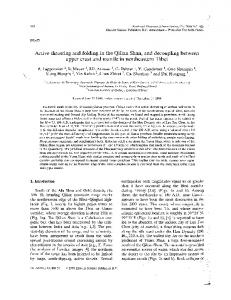
Fig. 2. Debiased cumulative surface density of TNOs for G01 (open squares), P0 (open diamonds), and MEGAPrime data of F07 (open circles). The data have been debiased using the published efficiency functions. The different lines represent the best-fit singleexponential LF for G01 (dotted line), P06 (dash-dotted line), and F07 (dashed line). All three surveys, taken independently, are well approximated by a single exponential function with index ranging from 0.7 to 0.8. Clearly, one cannot simply combine them as was done up to and including B04 (although CB99 noted that combining leads to inconsistent results). One must account for an offset in surface density due to longitude and latitude variation, magnitude difference in different passband filters, and calibration uncertainties. An attempt to apply these corrections was done by F07, but this requires external determination of these offset in order to avoid unreasonable fit values for m0 for surveys with small number of detections (F07).

dynamical class. Thus, few people tried to address this question, and most of those who did assumed a unique size distribution for all classes, with only a change in the normalizing factor. JLT98 had to assume some orbital distribution of objects to solve for the size distribution. They used a two-population model composed of a classical Kuiper belt and Plutinos. In doing so, they used the same size distribution form for both populations, and assumed a simplified model of the semimajor axis and eccentricity distributions of the classical belt, as well as the eccentricity distribution of the Plutinos. In doing so, they estimated that the apparent Plutino fraction of ~38% found in their data corresponds to a 10–20% fraction of the TNOs in the 30–50-AU region. Furthermore, they computed the bias in their survey against finding objects in the 2:1 resonance with Neptune and concluded that the nondetection of those could not formally disprove the hypothesis that the 2:1 and 3:2 resonances are equally populated (Malhotra, 1995). Note that the classification used

rather short arcs, typically 1 year or less for many objects in the survey, which may lead to misclassification. TJL01 applied the same approach to their new survey, for which they attempted to obtain better orbital determination by longer tracking effort. Using the bias toward finding 3:2 resonant objects computed by JLT98, they converted their observed 8% Plutino fraction to a 3–4% real fraction, much smaller than the previous estimate, and more in line with the findings of Petit and Gladman (2003). As for the 2:1 population, their conclusions were similar to those of JLT98. L00 used also a single slope for their LF for all TNOs and give their sky density of classical belt and of scattering (scattered in their paper) disk and find the latter to be about six times less populated than the former. They also considered what they called Centaurs (not a population of TNOs per se), of which they discovered four, and derived a shallower slope than for TNOs, and a much lower sky density of 0.017 ± 0.011 Centaurs brighter than mR = 21.5. However, according to the new classification scheme KBB07


described in the chapter by Gladman et al., only two objects are Centaurs, one (1998 SG35 = Okyrhoe) is a JFC, and the last one (33128=1998 BU48) is a scattered disk object. We note that the objects used in that work typically had a decently determined orbit, and the change in classification is due to the fuzzy definitions used at that time. T01 confirmed the sky density of Centaurs at the bright end, finding one such object (using the same definition as L00) in their survey. B04 were the first to try and fit completely different LFs to different dynamical classes. They define three different classes that span one or more classes of KBB07. The TNO sample contains all objects with heliocentric distance R > 25 AU. The CKBO sample roughly correspond to the classical belt, with 38 AU < R < 55 AU and inclination i < 5°. The excited sample is the complement of the CKBOs in the TNOs. They find that the differential LF of the CKBO sample is well described by a very steep slope (α ~ 1.4) at the bright end, and a shallower, but still rising, slope (α ~ 0.4) at the faint end, while the differential LF of the excited sample would have a bright end slope similar to that derived by other works to the whole belt (α ~ 0.65), and would be decreasing at the faint end (slope α ~ –0.5). This result is to be taken with great caution as the classification used was purely practical and has no connection to any common (or lack of) origin of the bodies. E05 had the best survey at the time to address the question of size distribution vs. dynamical population, having the largest number of objects discovered in a single survey. They were also able to determine precisely the orbit of a fair fraction of their objects. They consider three major classes of TNOs — mainly the classical belt, the resonant objects, and the scattered objects — with boundaries similar to those of KBB07. They find that the slope of the LF varies significantly from the classical belt (0.72), to the resonant objects (0.60), to the scattered objects (1.29). Interestingly, the slope of their overall sample is steeper (0.88) than for any subsample but the scattered one, which make up only a small fraction of the objects. However, a caveat is in order here, since E05 did not actually measure their efficiency at discovery, but rather used a heuristic approach to estimate it. Also, only about half of their objects had an orbit precise enough to allow for classification. 7.

FUTURE WORK AND LINK WITH FORMATION AND COLLISIONAL EVOLUTION MODELS

The two major outstanding issues on this topic concern the size distribution of the various dynamical classes and the size(s) at which the shape of the distribution changes. The work of B04 has shown that, going to the faint end of the LF, there is a knee in the size distribution, which they estimate to be around mR ~ 24–25. But P06 and F07 have shown the straight exponential to extend to at least mR = 26. To settle this question, we will need a deg2 survey down to R magnitude 28 or so, beyond the expected knee in the size distribution. At the other end of the LF, earlier works

85

(ITZ95, and to a lesser extend JLT98) have reported the need for a steeper slope of the LF for objects brighter than mR ~ 22–23. ITZ95 were the only ones to give an estimate of the needed slope, at 1.5. All subsequent works assumed a single slope brightward of mR ~ 24–25. However, these works were dealing mostly with LF faintward of mR ~ 22, either explicitly or implicitly. Deciding if there is really a change in the LF slope brightward of mR ~ 22–23 requires surveying the ~1500 deg2 around the ecliptic plane where the classical Kuiper belt resides, down to R magnitude 22–23. The challenge for determining the size distribution of the different dynamical classes is that we need to have a fully characterized survey finding a decent number of TNOs in each class, and follow them all (or at least a large fraction of them, without orbital bias) to firmly establish their class. This requires a follow-up program for at least 2 years after discovery. The only current survey of this kind is the Very Wide component of the CFHT Legacy Survey, which discovers TNOs as faint as mR = 23.5–24 depending on the seeing conditions. It has covered 300 deg2 in its discovery phase and is still chasing the objects it has discovered. The forthcoming Pan-STARRS survey will cover the entire sky to 0.5–1 mag fainter than the current CFHTLS-VW survey. Both can address the question of the size distribution for the large-sized bodies, larger than the transition knee detected by B04. In the 5 to 10 years to come, we should have a good knowledge of the size distribution of the large bodies (larger than 100 km in radius) in each of the main dynamical classes, allowing useful comparison with early accretion models. The size distribution of TNOs smaller than the knee for the CKBO class (the most abundant one in most of the surveys) will also be determined during the same period, thanks to large efforts on 8-m-class telescopes. Determining the shape of the size distribution of small TNOs in each dynamical class is the step after determining that of the TNOs as a whole. This will require a large sample in each dynamical class, hence surveying several deg2 of sky to be observed to magnitude ~28. All objects thus discovered will have to be followed until their orbit has been firmly established. This will occur only when we have deg2 cameras on either Extremely Large Telescopes or on the new generation of Space Telescopes. Acknowledgments. We thank M. Holman, S. Kenyon, A. Morbidelli, and an anonymous reviewer for comments that considerably improved the text. J-M.P. acknowledges support from CNRS and the Programme National de Planétologie.

REFERENCES Albrecht R., Barbieri C., Adorf H.-M., Corrain G., Gemmo A., Greenfield P., Hainaut O., Hook R. N., Tholen D. J., Blades J. C., and Sparks W. B. (1994) High-resolution imaging of the Pluto-Charon system with the Faint Object Camera of the Hubble Space Telescope. Astrophys. J. Lett., 435, L75–L78. Altenhoff W. J., Bertoldi F., and Menten K. M. (2004) Size estimates of some optically bright KBOs. Astron. Astrophys., 415, 771–775.

86


Benz W. and Asphaug E. (1999) Catastrophic disruptions revisited. Icarus, 142, 5–20. Bernstein G. M., Trilling D. E., Allen R. L., Brown M. E., Holman M., and Malhotra R. (2004) The size distribution of transneptunian bodies. Astron. J., 128, 1364–1390. Bowell E., Hapke B., Domingue D., et al. (1989) Application of photometric models to asteroids. In Asteroids II (R. P. Binzel et al., eds.), pp. 524–556. Univ. of Arizona, Tucson. Brown M. E. and Trujillo C. A. (2004) Direct measurement of the size of the large Kuiper Belt object (50000) Quaoar. Astron. J., 127, 2413–2417. Brown M. E., Schaller E. L., Roe H. G., Rabinowitz D. L., and Trujillo C. A. (2006) Direct measurement of the size of 2003 UB313 from the Hubble Space Telescope. Astrophys. J. Lett., 643, L61–L63. Bruzual G. and Charlot S. (2003) Stellar population synthesis at the resolution of 2003. Mon. Not. R. Astron. Soc., 344, 1000– 1028. Chiang E. I. and Brown M. E. (1999) Keck pencil-beam survey for faint Kuiper belt objects. Astron. J., 118, 1411–1422. Chiang E. I. and Jordan A. B. (2002) On the Plutinos and twotinos of the Kuiper belt. Astron. J., 124, 3430–3444. Cochran A. L., Levison H. F., Stern S. A., and Duncan M. J. (1995) The discovery of Halley-sized Kuiper belt objects using the Hubble Space Telescope. Astrophys. J., 455, 342–346. Cruikshank D. P., Stansberry J. A., Emery J. P., Fernández Y. R., Werner M. W., Trilling D. E., and Rieke G. H. (2005) The high-albedo Kuiper belt object (55565) 2002 AW197. Astrophys. J. Lett., 624, L53–L56. Davis D. R. and Farinella P. (1997) Collisional evolution of Edgeworth-Kuiper belt objects. Icarus, 125, 50–60. Dohnanyi J. S. (1969) Collisional model of asteroids and their debris. J. Geophys. Res., 74, 2531–2554. Drell P. S., Loredo T. J., and Wasserman I. (2000) Type Ia supernovae, evolution, and the cosmological constant. Astrophys. J., 530, 593–617. Drossart P. (1993) Optics on a fractal surface and the photometry of the regoliths. Planet. Space Sci., 41(5), 381–393. Elliot J. L., Kern S. D., Clancy K. B., Gulbis A. A. S., Millis R. L., Buie M. W., Wasserman L. H., Chang E. I., Jordan A. B., Trilling D. E., and Meech K. J. (2005) The Deep Ecliptic Survey: A search for Kuiper belt objects and Centaurs. II. Dynamical classification, the Kuiper belt plane, and the core population. Astron. J., 129, 1117–1162. Farinella P. and Davis D. R. (1996) Short-period comets: Primordial bodies or collisional fragments? Science, 273, 938– 941. Fukugita M., Shimasaku K., and Ichikawa T. (1995) Galaxy colors in various photometric band systems. Publ. Astron. Soc. Pac., 107, 945. Gault D. E., Shoemaker E. M., and Moore H. J. (1963) Spray Ejected from the Lunar Surface by Meteoroid Impact. NASA Rept. TND-1167, U.S. Govt. Printing Office, Washington, DC. Giblin I., Martelli G., Smith P. N., Cellino A., DiMartino M., Zappalà V., Farinella P., and Paolocchi P. (1994) Field fragmentation of macroscopic targets simulating asteroidal catastrophic collisions. Icarus, 110, 203–224. Giblin I., Martelli G., Farinella P., Paolicchi P., Di Martino M., and Smith P. N. (1998) The properties of fragments from catastrophic disruption events. Icarus, 134, 77–112. Gladman B., Kavelaars J. J., Nicholson P. D., Loredo T. J., and Burns J. A. (1998) Pencil-beam surveys for faint trans-neptunian objects. Astron. J., 116, 2042–2054.

Gladman B., Kavelaars J. J., Petit J.-M., Morbidelli A., Holman M. J., and Loredo T. (2001) The structure of the Kuiper belt: Size distribution and radial extent. Astron. J., 122, 1051–1066. Gregory P. G. (2005) Bayesian Logical Data Analysis for the Physical Sciences: A Comparative Approach with Mathematica Support. Cambridge Univ., Cambridge. Grundy W. M., Noll K. S., and Stephens D. C. (2005) Diverse albedos of small trans-neptunian objects. Icarus, 176, 184–191. Gull S. L. (1989) Bayesian data analysis — Straight line fitting. In Maximum Entropy and Bayesian Methods (J. Skilling, ed.), pp. 511–518. Kluwer, Dordrecht. Hapke B., Nelson R., and Smythe W. (1998) The opposition effect of the Moon: Coherent backscatter and shadow hiding. Icarus, 133, 89–97. Helfenstein P., Veverka J., and Hillier J. (1997) The lunar opposition effect: A test of alternative models. Icarus, 128, 2–14. Irwin M., Tremaine S., and Zytkow A. N. (1995) A search for slow-moving objects and the luminosity function of the Kuiper belt. Astron. J., 110, 3082–3092. Jeffreys H. (1961) Theory of Probability. Oxford Univ., Oxford. Jefferys W. H. and Berger J. O. (1992) Ockham’s Razor and Bayesian Analysis. Am. Sci., 80, 64–72. Jewitt D. and Luu J. (1993) Discovery of the candidate Kuiper belt object 1992 QB1. Nature, 362, 730–732. Jewitt D. and Luu J. X. (1995) The solar system beyond Neptune. Astron. J., 109, 1867–1876. Jewitt D., Luu J., and Chen J. (1996) The Mauna Kea-CerroTololo (MKCT) Kuiper belt and Centaur survey. Astron. J., 112, 1225–1238. Jewitt D. C., Luu J. X., and Trujillo C. (1998) Large Kuiper belt objects: The Mauna Kea 8k CCD survey. Astron. J., 115, 2125–2135. Kowal C. (1989) A solar system survey. Icarus, 77, 118–123. Lacerda P. and Luu J. (2006) Analysis of the rotational properties of Kuiper belt objects. Astron. J., 131, 2314–2326. Larsen J. A., Gleason A. E., Danzi N. M., Descour A. S., McMillan R. S., Gehrels T., Jedicke R., Montani J. L., and Scotti J. V. (2001) The Spacewatch wide-area survey for bright Centaurs and trans-neptunian objects. Astron. J., 121, 562–579. Levison H. F. and Duncan M. J. (1990) A search for proto-comets in the outer regions of the solar system. Astron. J., 100, 1669– 1675. Levison H. F. and Duncan M. J. (1997) From the Kuiper belt to Jupiter-family comets: The spatial distribution of ecliptic comets. Icarus, 127, 13–32. Loredo T. J. (2004) Accounting for source uncertainties in analyses of astronomical survey data. In Bayesian Inference and Maximum Entropy Methods in Science and Engineering (R. Fischer et al., eds.), pp. 195–206. AIP Conference Proceedings 735, American Institute of Physics, New York. Loredo T. J. and Lamb D. Q. (2002) Bayesian analysis of neutrinos observed from supernova SN 1987A. Phys. Rev. D, 65, 063002. Loredo T. J. and Wasserman I. M. (1995) Inferring the spatial and energy distribution of gamma-ray burst sources. I. Methodology. Astrophys. J. Suppl., 96, 261–301. Luu J. X. and Jewitt D. (1988) A two-part search for slow-moving objects. Astron. J., 95, 1256–1262. Luu J. X. and Jewitt D. (1998) Deep imaging of the Kuiper belt with the Keck 10 meter telescope. Astrophys. J. Lett., 502, L91–L94. Malhotra R. (1995) The origin of Pluto’s orbit: Implications for the solar system beyond Neptune. Astron. J., 110, 420–429.


Malhotra R. (1996) The phase space structure near Neptune resonances in the Kuiper belt. Astron. J., 111, 504–516. Morbidelli A. and Brown M. E. (2004) The Kuiper belt and the primordial evolution of the solar system. In Comets II (M. C. Festou et al., eds.), pp. 175–191. Univ. of Arizona, Tucson. Petit J.-M. and Gladman B. (2003) Discovering and securing TNOs: The CFHTLS ecliptic survey. C. R. Phys., 4, 743–753. Petit J.-M. and Mousis O. (2004) KBO binaries: How numerous were they? Icarus, 168, 409–419. Petit J.-M., Holman M. J., Gladman B. J., Kavelaars J. J., Scholl H., and Loredo T. J. (2006) The Kuiper belt’s luminosity function from mR = 22–25. Mon. Not. R. Astron. Soc., 365, 429– 438. Rousselot P., Belskaya I. N., and Petit J.-M. (2006) Do the phase curves of KBOs present any correlation with their physical and orbital parameters? Bull. Am. Astron. Soc., 38, 44.08. Ryan E. V., Davis D. R., and Giblin I. (1999) A laboratory impact study of simulated Edgeworth-Kuiper belt objects. Icarus, 142, 56–62. Schaefer B. E. and Rabinowitz D. L. (2002) Photometric light curve for the Kuiper belt object 2000 EB173 on 78 nights. Icarus, 160, 52–58. Sheppard S. S. and Jewitt D. C. (2002) Time-resolved photometry of Kuiper belt objects: Rotations, shapes, and phase functions. Astron. J., 124, 1757–1775.

87

Sheppard S. S., Jewitt D. C., Trujillo C. A., Brown M. J. I., and Ashley M. B. C. (2000) A wide-field CCD survey for Centaurs and Kuiper belt objects. Astron. J., 120, 2687–2694. Shkuratov Y. G. and Helfenstein P. (2001) The opposition effect and the quasi-fractal structure of regolith: I. Theory. Icarus, 152, 96–116. Sivia D. and Skilling J. (2006) Data Analysis: A Bayesian Tutorial, second edition. Oxford Univ., New York. Stansberry J. A., Grundy W. M., Margot J. L., Cruikshank D. P., Emery J. P., Rieke G. H., and Trilling D. E. (2006) The albedo, size, and density of binary Kuiper belt object (47171) 1999 TC36. Astrophys. J., 643, 556–566. Tombaugh C. W. (1961) The trans-neptunian planet search. In Planets and Satellites (G. P. Kuiper and B. M. Middlehurst, eds), pp. 12–30. Univ. of Chicago, Chicago. Trujillo C. A. and Brown M. E. (2001) The radial distribution of the Kuiper belt. Astrophys. J. Lett., 554, L95–L98. Trujillo C. A., Jewitt D. C., and Luu J. X. (2001a) Properties of the trans-neptunian belt: Statistics from the Canada-France-Hawaii Telescope survey. Astron. J., 122, 457–473. Trujillo C. A., Luu J. X., Bosh A. S., and Elliot J. L. (2001b) Large bodies in the Kuiper belt. Astron. J., 122, 2740–2748. Wasserman L. (1997) Carnegie Mellon University Dept. of Statistics Technical Report 666. Carnegie Mellon Univ., Pittsburgh.

88


Size Distribution of Multikilometer Transneptunian Objects - Caltech GPS

Size Distribution of Multikilometer Transneptunian Objects - Caltech GPS

Suggest Documents

Transneptunian Object Taxonomy - Caltech GPS

Retrieval of stratospheric aerosol size distribution from ... - Caltech GPS

Polarimetry of transneptunian objects (136472) Makemake and ...

Photometric Lightcurves of Transneptunian Objects and Centaurs ...

The Size Distribution of Kuiper Belt Objects

Stromboli - Caltech GPS

1. INTRODUCTION - Caltech GPS

Seismo#678 - Caltech GPS

sem2dpack - Caltech GPS

1295 - Caltech GPS

Untitled - Caltech GPS

science letters - Caltech GPS

DOC006 - Caltech GPS

SATURN'S RINGS - Caltech GPS

letters - Caltech GPS

1221 - Caltech GPS

Reconfigurable Computing - Caltech GPS

perspectives - Caltech GPS

som - Caltech GPS

perspectives - Caltech GPS

features - Caltech GPS

â¢ 35 - Caltech GPS

letters - Caltech GPS

Elemental Sulfur - Caltech GPS

Size Distribution of Multikilometer Transneptunian Objects - Caltech GPS