C = Centaurs, Cl = classical, R = resonant, S = scattered ..... and Centaur the respective taxon and the number of colors (N) used in classifying it are reported.
Fulchignoni et al.: Transneptunian Object Taxonomy
181
Transneptunian Object Taxonomy Marcello Fulchignoni LESIA, Observatoire de Paris
Irina Belskaya Kharkiv National University
Maria Antonietta Barucci LESIA, Observatoire de Paris
Maria Cristina De Sanctis IASF-INAF, Rome
Alain Doressoundiram LESIA, Observatoire de Paris
A taxonomic scheme based on multivariate statistics is proposed to distinguish groups of TNOs having the same behavior concerning their BVRIJ colors. As in the case of asteroids, the broadband spectrophotometry provides a first hint about the bulk compositional properties of the TNOs’ surfaces. Principal components (PC) analysis shows that most of the TNOs’ color variability can be accounted for by a single component (i.e., a linear combination of the colors): All the studied objects are distributed along a quasicontinuous trend spanning from “gray” (neutral color with respect to those of the Sun) to very “red” (showing a spectacular increase in the reflectance of the I and J bands). A finer structure is superimposed to this trend and four homogeneous “compositional” classes emerge clearly, and independently from the PC analysis, if the TNO sample is analyzed with a grouping technique (the G-mode statistics). The first class (designed as BB) contains the objects that are neutral in color with respect to the Sun, while the RR class contains the very red ones. Two intermediate classes are separated by the G mode: the BR and the IR, which are clearly distinguished by the reflectance relative increases in the R and I bands. Some characteristics of the classes are deduced that extend to all the objects of a given class the properties that are common to those members of the class for which more detailed data are available (observed activity, full spectra, albedo). The distributions of the classes with respect to the distance from the Sun and to the orbital inclination give some hints on the chemico-physical structure of the inner part of the Kuiper belt. An interpretation of the average broadband spectra of the four classes as the result of modifying processes (collisions, space weathering, degassing, etc.), allows us to read the proposed taxonomy in terms of the evolution of TNOs.
1.
INTRODUCTION
Taxonomy (from the Greek verb τασσει’ν or tassein = “to classify” and νο′μος or nomos = “law, science”) was once only the science of classifying living organisms (alpha taxonomy), but later the word was applied in a wider sense, and may also refer to either a classification of things, or the principles underlying the classification. Almost anything — animate objects, inanimate objects, places, and events — may be classified according to some taxonomic scheme. Such an approach to studying physical properties
became an efficient tool in asteroid investigations, which enabled the expansion of our knowledge of physical properties of well-studied asteroids within a taxon to other members belonging to the same taxon. Multivariate and canonical (parametrical and/or nonparametrical) analysis of the color distribution of transneptunian objects (TNOs) and associated families and their orbital parameters, together with recently developed cluster analysis methods, could be used in order to set the basis of taxonomy. The objectives are to demonstrate, rule out, or constrain the several dynamical, thermal, and surface evolution mod-
181
182
The Solar System Beyond Neptune
els and characterize the several dynamical subclasses of TNOs by their surface and orbital properties, defining or constraining their boundaries. Wood and Kuiper (1963) suggested, on the basis of the distribution of about 40 asteroids in the U–B and B–V plot, the existence of two different compositional classes clustering around the color indices of the Moon and the Sun. These groups were the ancestors of the currently used asteroid S and C classes, respectively. Tholen and Barucci (1989) summarized the results of their asteroid taxonomies for about 400 asteroids obtained by means of independent multivariate statistical techniques [the principal components (PC) analysis based on eightcolor data from Zellner et al. (1985) and the G-mode analysis based on the same eight colors database to which the IRAS albedo data from Tedesco et al. (1992) were added]. Tedesco et al. (1989) obtained three-parameter taxonomy analyzing more than 350 asteroids described by two colors indices (U–V and v–x) and the visual albedo. All these methods provided a similar classification scheme separating the asteroid population into a dozen compositionally homogeneous groups, as outlined by Barucci and Fulchignoni (1990). Analyzing the B–V and V–R colors of 13 TNOs and Centaurs, Tegler and Romanishin (1998) obtained two groups, one very red and the other quite neutral with respect to the Sun. Barucci et al. (2001) applied both techniques used in classifying the asteroids to a sample of 22 TNOs and Centaurs characterized by four colors (B–V, V–R, V–I, and V– J). The results indicate a clear compositional trend within the examined sample and suggest the possible existence of four homogeneous groups. The increase of the available data allowed Fulchignoni et al. (2003) and Barucci et al. (2005a) to confirm this result at a higher significance level, analyzing samples of 34 and 51 objects respectively. An interesting attempt to characterize the TNOs on the basis of their orbital elements and some physical properties has been recently carried out by De Sanctis et al. (2006), who used the G mode to analyze 81 TNOs chosen among those with well-known dynamical parameters, described by the color indices B–V and V–R, the absolute magnitude H, the orbital inclination i, orbital eccentricity e, and semimajor axis a. The G-mode analysis separates the 81 objects of the sample in five groups, well separated for the dynamical parameters and less separated in colors. The obtained groups are close to the well-known dynamical ones (classical, Plutinos, scattered, and detached), but the classification firmly identifies two different types of classical objects, corresponding to the “so-called” dynamically cold and hot classical population. Moreover, they found trends and correlations within the members of the different groups. To distinguish groups of objects with similar properties we need to have a statistically representative dataset. However, the knowledge of physical properties of TNOs is still very limited: To date, the available information concerning TNOs include (1) orbital parameters (known for all the objects with different degrees of precision) and (2) broadband
B, V, R, I photometry for about 130 objects; for approximately 70 of them J data are also available, while H and K photometry has been obtained for only about 55 of them. Hereafter we present the first taxonomic scheme used to obtain a classification of the TNOs. In fact, when dealing with a large number of objects, it is very important to distinguish groups of objects with similar properties, preferably based on measured common characteristics. 2. DATA AND STATISTICAL METHODS We successively analyzed two homogeneous TNO samples: (1) 67 objects described by four color indices (B–V, V–R, V–I, V–J); (2) 55 objects described by six color indices (B–V, V–R, V–I, V–J, V–H, V–K). The list of objects and their colors together with the references to the original data are given in Table 1. When multiple observations of an object were available, for the colors we adopted their mean values weighted with the inverse of the error of individual measurement and the standard deviation was assumed as the error. In the case of a single measurement we restricted our consideration to those objects for which colors were determined with an error less than 0.1 mag for BVRIJ colors. The selected data represent a homogeneous dataset in B, V, R, I, J, H, and K bands in general obtained by the same observer during the same run, or intercalibrated through the V measurements. We used nonsimultaneous V and the JHK set of magnitudes in a few cases when it was possible to recalculate V magnitude to the epoch of JHK measurements taking into account the geometry of observations. The analysis has been carried out using both principal component analysis (PCA) (Reyment and Joreskog, 1993) and G-mode analysis (Coradini et al., 1977; Fulchignoni et al., 2000). The principal components (PC) are linear combinations of the original variables whose coefficients reflect the relative importance of each variable (color) within each principal component. These coefficients are the eigenvectors of the variance-covariance matrix of the colors. The sum of the eigenvalues of this matrix (which is equal to its trace) accounts for the total variance of each sample. Each eigenvalue reflects the percentage of the total variance contributed by each principal component. We analyzed the same samples with the G-mode multivariate statistics (Coradini et al., 1977), which allowed us to investigate the existence of a finer structure of the samples. G-mode statistics were applied to our samples of 67 and 55 objects described by four and six variables, respectively. The total number of degrees of freedom (268 and 330 respectively) allow us to use this type of statistics. The goal of the analysis is to find groups of objects that have a homogeneous behavior, if any, in terms of their physical characteristics (variables) under consideration. The method provides a quantitative estimation of the weight of each variable in separating the groups. We refer the reader to the quoted literature for details on both PC and G-mode statistics.
Sun 2060 Chiron/C 5145 Pholus/C 7066 Nessus/C 8405 Asbolus/C 10199 Chariklo/C 10370 Hylonome/C 15788 1993 SB/R 15789 1993 SC/R 15820 1994 TB/R 15874 1996 TL66/S 15875 1996 TP66/R 19299 1996 SZ4/R 19308 1996 TO66/Cl 19521 Chaos/Cl 20000 Varuna/Cl 24835 1995 SM55/Cl 24952 1997 QJ4/R 26181 1996 GQ21/R 26308 1998 SM165/R 26375 1999 DE9/S 28978 Ixion/R 29981 1999 TD10/S 31824 Elatus/C 32532 Thereus/C 32929 1995 QY9/R 33128 1998 BU48/S 33340 1998 VG44/R 35671 1998 SN165/Cl 38628 Huya/R 40314 1999 KR16/D 42301 2001 UR163/R 42355 2002 CR46/S 44594 1999 OX3/S 47171 1999 TC36/R 47932 2000 GN171/R 48639 1995 TL8/Cl 52872 Okyrhoe/JFC 52975 Cyllarus/C 54598 Bienor/S 55565 2002 AW197/Cl
Object/Type*
0.67 0.63 ± 0.02 1.25 ± 0.03 1.09 ± 0.01 0.75 ± 0.01 0.80 ± 0.02 0.69 ± 0.06 0.80 ± 0.02 1.08 ± 0.08 1.10 ± 0.02 0.73 ± 0.03 1.05 ± 0.06 0.75 ± 0.08 0.67 ± 0.03 0.94 ± 0.03 0.88 ± 0.02 0.65 ± 0.01 0.76 ± 0.04 1.01 ± 0.01 0.98 ± 0.02 0.97 ± 0.03 1.03 ± 0.03 0.75 ± 0.02 1.03 ± 0.03 0.75 ± 0.01 0.70 ± 0.02 0.95 ± 0.08 0.90 ± 0.01 0.71 ± 0.06 0.96 ± 0.02 1.06 ± 0.03 1.30 ± 0.11 0.83 ± 0.07 1.15 ± 0.02 1.03 ± 0.02 0.92 ± 0.01 1.04 ± 0.01 0.75 ± 0.04 1.13 ± 0.04 0.69 ± 0.02 0.90 ± 0.03
B–V 0.36 0.35 ± 0.01 0.77 ± 0.01 0.79 ± 0.01 0.47 ± 0.02 0.48 ± 0.01 0.43 ± 0.02 0.47 ± 0.01 0.70 ± 0.06 0.69 ± 0.02 0.37 ± 0.02 0.66 ± 0.02 0.52 ± 0.03 0.40 ± 0.02 0.62 ± 0.01 0.61 ± 0.02 0.38 ± 0.02 0.43 ± 0.06 0.71 ± 0.01 0.65 ± 0.04 0.58 ± 0.01 0.61 ± 0.03 0.49 ± 0.02 0.66 ± 0.01 0.49 ± 0.02 0.51 ± 0.04 0.64 ± 0.02 0.59 ± 0.01 0.42 ± 0.03 0.57 ± 0.02 0.76 ± 0.01 0.84 ± 0.01 0.55 ± 0.05 0.69 ± 0.02 0.69 ± 0.01 0.62 ± 0.01 0.69 ± 0.01 0.47 ± 0.02 0.69 ± 0.01 0.47 ± 0.02 0.62 ± 0.03
V–R 0.69 0.70 ± 0.04 1.58 ± 0.01 1.47 ± 0.03 0.98 ± 0.01 1.01 ± 0.01 0.96 ± 0.03 1.01 ± 0.01 1.49 ± 0.04 1.43 ± 0.03 0.72 ± 0.01 1.31 ± 0.07 0.97 ± 0.14 0.75 ± 0.02 1.19 ± 0.05 1.24 ± 0.02 0.71 ± 0.02 0.81 ± 0.05 1.42 ± 0.01 1.30 ± 0.01 1.15 ± 0.01 1.19 ± 0.04 1.02 ± 0.03 1.28 ± 0.01 0.94 ± 0.01 0.86 ± 0.06 1.18 ± 0.01 1.18 ± 0.08 0.82 ± 0.01 1.20 ± 0.02 1.50 ± 0.03 1.46 ± 0.11 0.99 ± 0.06 1.39 ± 0.02 1.33 ± 0.02 1.22 ± 0.02 1.33 ± 0.01 0.97 ± 0.02 1.36 ± 0.03 0.92 ± 0.05 1.18 ± 0.03
V–I 1.08 1.13 ± 0.01 2.57 ± 0.03 2.29 ± 0.01 1.65 ± 0.02 1.73 ± 0.03 1.32 ± 0.01 1.43 ± 0.11 2.42 ± 0.07 2.37 ± 0.09 1.46 ± 0.10 2.26 ± 0.08 1.87 ± 0.13 1.00 ± 0.10 1.89 ± 0.03 1.99 ± 0.01 1.07 ± 0.05 1.23 ± 0.31 2.39 ± 0.04 2.36 ± 0.01 1.84 ± 0.04 1.88 ± 0.09 1.88 ± 0.07 2.09 ± 0.07 1.69 ± 0.05 2.02 ± 0.01 2.27 ± 0.05 1.81 ± 0.01 1.27 ± 0.05 1.95 ± 0.02 2.37 ± 0.10 2.37 ± 0.06 1.83 ± 0.09 2.20 ± 0.05 2.32 ± 0.01 1.84 ± 0.08 2.42 ± 0.05 1.93 ± 0.10 2.42 ± 0.07 1.74 ± 0.03 1.82 ± 0.06
V–J
± ± ± ± ± ± ±
2.88 2.91 2.17 2.18 2.31 2.48 2.14
± ± ± ± ± ± ± ± ± ± ± ±
0.05 0.12 0.08 0.12 0.05 0.03 0.14 0.09 0.12 0.11 0.05 0.08
2.34 2.63 2.70 2.38 2.80 2.52 2.77 2.27 2.38
± ± ± ± ± ± ± ± ±
0.09 0.10 0.02 0.14 0.09 0.10 0.11 0.11 0.10
2.37 ± 0.06 2.97 ± 0.12
0.08 0.07 0.05 0.09 0.10 0.09 0.05
2.27 2.95 2.86 2.18 2.63 2.70 2.21 2.82 2.40 2.87 2.14 2.15
± ± ± ± ± ± ±
0.18 0.04 0.08 0.05
2.60 ± 0.11 2.23 ± 0.01
3.03 2.96 2.19 1.97 2.43 2.51 2.30
± ± ± ±
2.79 ± 0.11 2.21 ± 0.01
0.04 0.02 0.05 0.11 0.10 0.09 0.07
0.20 0.03 0.07 0.06
1.60 2.32 2.52 0.49
± ± ± ±
0.20 0.09 0.15 0.08
0.79 2.29 2.55 0.59
± ± ± ±
2.78 2.93 1.77 2.44
± ± ± ±
2.82 2.78 1.81 2.42
0.21 0.09 0.17 0.08
1.43 1.50 ± 0.03 2.93 ± 0.04 2.57 ± 0.10 2.22 ± 0.08 2.21 ± 0.03 1.77 ± 0.09
V–K
1.37 1.43 ± 0.01 2.94 ± 0.04 2.57 ± 0.10 2.06 ± 0.04 2.14 ± 0.03 1.50 ± 0.08
V–H
TABLE 1. Average colors of the selected sample objects.
1,2 14,15,16,17,46 8,15,16,17,46 14,15,16,17 15,16,17,18,19 3,5,16,17,42 5,9,15,16,17,42 3,4,6,20,22,23 3,4,7,8,14, 3,4,8,9,11,12,20,46 3,4,5,7,10,46 3,4,5,7,9,10,46 3,4,22,24 3,5,7,10,25,26,27 4,9,10,11,12,22,46 4,9,13,28,46 4,6,9,10,11,12,28,46 3,4,6,20,24 11,13,24,29,46 4,11,12,22,46 3,9,11,20,29,30,46 46 4,20,28,46 9,12,17,28, 46 17,31,32,46 4,6,9,14 9,11,12,13,17 4,9,10,46 3,4,6,9,20 3,4,9,24,28,33,34,46 3,11,13,36 43,46 46 4,9,17,22,35,43,46 4,9,10,11,12,30,41,46 4,13,24,46 11,20 9,17,20,28,41,46 9,10,11,12,17 9,11,12,17,30,41,46 39
References
Fulchignoni et al.: Transneptunian Object Taxonomy
183
1.11 0.94 0.99 0.85 0.72 0.82 1.08 0.87 0.87 1.10 0.77 1.23 0.68 0.72 0.73 1.19 1.05 0.63 0.71 1.06 0.78 0.86 0.82 0.75 0.60 0.65 0.61
± ± ± ± ± ± ± ± ± ± ± ± ± ± ± ± ± ± ± ± ± ± ± ± ± ± ±
0.01 0.06 0.01 0.08 0.05 0.17 0.03 0.03 0.06 0.04 0.05 0.09 0.04 0.05 0.06 0.02 0.06 0.03 0.02 0.03 0.03 0.01 0.06 0.04 0.15 0.02 0.08
B–V 0.71 0.54 0.73 0.47 0.48 0.65 0.66 0.39 0.58 0.76 0.38 0.76 0.37 0.49 0.51 0.66 0.67 0.34 0.45 0.73 0.53 0.52 0.60 0.33 0.50 0.36 0.45
± ± ± ± ± ± ± ± ± ± ± ± ± ± ± ± ± ± ± ± ± ± ± ± ± ± ±
0.01 0.06 0.06 0.01 0.03 0.06 0.04 0.02 0.04 0.01 0.05 0.09 0.04 0.03 0.04 0.03 0.05 0.02 0.02 0.03 0.04 0.02 0.05 0.06 0.10 0.02 0.07
V–R 1.38 1.13 1.29 0.94 1.06 1.30 1.25 1.07 1.07 1.44 1.36 1.37 0.74 0.88 0.92 1.44 1.27 0.68 0.78 1.31 0.99 1.10 1.22 0.75 0.80 0.76 0.80
± ± ± ± ± ± ± ± ± ± ± ± ± ± ± ± ± ± ± ± ± ± ± ± ± ± ±
0.05 0.05 0.03 0.02 0.03 0.06 0.03 0.03 0.05 0.01 0.08 0.09 0.04 0.01 0.05 0.14 0.07 0.02 0.02 0.08 0.03 0.04 0.08 0.08 0.15 0.06 0.07
V–I 2.14 1.82 1.84 1.49 1.65 2.01 2.06 1.68 1.92 2.46 1.48 2.32 1.08 1.57 1.63 2.41 1.98 1.05 1.01 1.87 1.67 1.86 2.42 1.65 1.53 1.30 1.46
± ± ± ± ± ± ± ± ± ± ± ± ± ± ± ± ± ± ± ± ± ± ± ± ± ± ±
0.03 0.09 0.37 0.10 0.07 0.07 0.03 0.12 0.12 0.02 0.07 0.06 0.04 0.09 0.08 0.08 0.10 0.02 0.02 0.03 0.04 0.07 0.08 0.08 0.10 0.10 0.10
V–J
(continued).
0.07 0.11 0.08 0.14 0.14 0.14
± ± ± ± ± ±
0.08 0.12 0.11 0.14 0.15 0.16
± ± ± ± ± ±
2.30 2.88 2.09 2.08 1.53 1.48
2.33 2.92 2.32 2.24 1.69 1.39
2.33 ± 0.16 0.94 ± 0.05 0.32 ± 0.05
± ± ± ±
2.26 1.01 0.72 2.52
0.14 0.04 0.04 0.08
2.19 ± 0.10
2.08 ± 0.10
0.11 0.09 0.09 0.09 0.16 0.16 0.02
2.66 ± 0.07 1.25 ± 0.04
± ± ± ± ± ± ±
2.39 2.26 2.59 2.48 2.18 2.39 2.79
0.12 0.09 0.11 0.08 0.16 0.17 0.02 0.11 0.06 0.04
2.05 2.02 2.49 2.44 2.02 2.09 2.83 2.09 2.61 1.21
± ± ± ± ± ± ± ± ± ±
2.37 ± 0.03 2.22 ± 0.11
V–K
2.44 ± 0.03 2.22 ± 0.10
V–H
39,46 46 3,6,9,10,25 12,17,24 17,29,30,35 4,11,20,37 3,4,5,9,10,11 46 46 39,46 46 21 40 4,9,10 46 3,4,5,6 9,11 45 44 3,4,5,7 38 11,12 9,11,12 9,11,12,46 11,13 11,43,46 46
References
References: [1] Hardlop (1980); [2] Hartmann et al. (1982); [3] Jewitt and Luu (2001); [4] McBride et al. (2003); [5] Tegler and Romanishin (1998); [6] Gil-Hutton and Licandro (2001); [7] Jewitt and Luu (1998); [8] Tegler and Romanishin (1997); [9] Doressoundiram et al. (2002); [10] Boehnhardt et al. (2001); [11] Delsanti et al. (2006); [12] Delsanti et al. (2004); [13] Sheppard and Jewitt (2002); [14] Luu and Jewitt (1996); [15] Davies et al. (1998); [16] Davies et al. (2000); [17] Bauer et al. (2003); [18] Romanishin et al. (1997); [19] RomonMartin et al. (2002); [20] Delsanti et al. (2001); [21] Barucci et al. (2005b); [22] Tegler and Romanishin (2000); [23] Davies et al. (1997); [24] Boehnhardt et al. (2002); [25] Davies (2000); [26] Hainaut et al. (2000); [27] Barucci et al. (1999); [28] Tegler and Romanishin (2003); [29] Doressoundiram et al. (2003); [30] Tegler et al. (2003); [31] Barucci et al. (2002); [32] Farnham and Davies (2003); [33] Ferrin et al. (2001); [34] Schaefer and Rabinowitz (2002); [35] Peixinho et al. (2004); [36] Trujillo and Brown (2002); [37] Doressoundiram et al. (2001); [38] Davies et al. (2001); [39] Doressoundiram et al. (2005a); [40] De Bergh et al. (2005); [41] Dotto et al. (2003); [42] McBride et al. (1999); [43] Doressoundiram et al. (2005b); [44] Brown et al. (2005); [45] Trujillo et al. (2007); [46] Doressoundiram et al. (2007).
*Type (from the chapter by Gladman et al.): C = Centaurs, Cl = classical, R = resonant, S = scattered, D = detached, JFC = Jupiter-family comet orbit, ? = unusual, Halley-family comet.
55576 Amycus/C 55637 2002 UX25/Cl 58534 Logos/Cl 60558 Echeclus/JFC 63252 2001 BL41/C 66652 1999 RZ253/Cl 79360 1997 CS29/Cl 82075 2000 YW134/R 82155 2001 FZ173/S 83982 Crantor/C 87555 2000 QB243/S 90377 Sedna/D 90482 Orcus/R 91133 1998 HK151/R 95626 2002 GZ32/C 118228 1996 TQ66 / R 134860 2000 OJ67/Cl 136108 2003 EL61/Cl 136199 Eris/D 1996 TS66/Cl 1998 WU24/? 1999 CD158/R 2000 OK67/Cl 2000 PE30/D 2001 CZ31/Cl 2001 QF298/R 2003 AZ84/R
Object/Type*
TABLE 1.
184 The Solar System Beyond Neptune
Fulchignoni et al.: Transneptunian Object Taxonomy
185
TABLE 2. Eigenvectors, eigenvalues, and percentage of total variance contributed by each eigenvalue from the PC analysis of the samples of 67 and 55 TNOs. Sample of 67 TNOs Variable B–V V–R V–I V–J Eigenvalues Percentage of total variance
1
2
3
4
0.311 0.235 0.450 0.804 0.269 92.892
0.508 0.241 0.579 –0.591 0.015 5.220
0.674 0.290 –0.678 0.034 0.004 1.269
–0.436 0.896 –0.054 –0.063 0.002 0.619
Sample of 55 TNOs Variable B–V V–R V–I V–J V–H V–K Eigenvalues Percentage of total variance
3.
1
2
3
4
5
6
0.147 0.116 0.234 0.440 0.605 0.592 0.880 93.312
0.427 0.280 0.477 0.413 –0.076 –0.579 0.044 4.664
0.332 0.167 0.405 –0.287 –0.578 0.530 0.011 1.199
–0.406 –0.006 –0.134 0.713 –0.530 0.166 0.004 0.409
0.721 –0.314 –0.569 0.202 –0.111 0.070 0.003 0.304
0.035 0.884 –0.461 –0.057 –0.011 0.032 0.001 0.112
RESULTS
We applied PCA successively to the dataset of 67 TNOs described by 4 variables (B–V, V–R, V–I, and V–J color indices) and to the subset of 55 TNOs described by 6 variables (B–V, V–R, V–I, V–J, V–H, and V–K color indices). The eigenvectors, percentages of total variance contributed by each eigenvector, and eigenvalues of the variance-covariance matrix of the two analyzed samples are reported in Table 2. These data show that in both cases (the results of the PC analysis carried out on 67 and 55 samples respectively) the first principal component (PC1) accounts for most of the variance of the sample (93%); the second principal component (PC2) adds only 4–5% to the total variance. The first and the second principal components account for about 98% of the total variance, therefore the PC1 vs. PC2 plane contains practically all the information on the variance of the variables characterizing the considered sample. This analysis establishes the existence of a quasicontinuous trend from neutral to very red objects along the PC1 axis. It is also possible to infer from these results that the degree of reddening is the main distinctive character of the TNO population. The predominance of PC1 (i.e., of V–I and V–J colors in the first case and V–H and V–K colors in the second one) in characterizing TNO behavior is shown by the PC1 scores, which span three times more than PC2. The objects having a neutral color with respect to the Sun have the lower values of the PC1 scores and fall in the left part of the histogram shown in Fig. 1; for larger PC1 scores the
objects are redder and redder. The object number density along the PC1 is not homogeneous, indicating the presence of some grouping that overlaps the continuous trend. In Fig. 1 the histogram represents the number of the objects projected onto the PC1, clearly showing four peaks. These groups of objects constitute a finer structure overlapping the general trend from neutral to very red spectra resulting from the PC analysis.
Fig. 1. Histogram showing the distribution of TNOs vs. the PC1 scores. The four superimposed curves represent the four classes obtained by the G mode. The Gaussians described by the parameters characterizing each class (average, standard deviation, and number of objects as reported in Table 3) are projected on the PC1 axis.
186
The Solar System Beyond Neptune
The relationship between the variables used is probably nonlinear, so the PC analysis does not allow us to discriminate among the intrinsic structure of these groups. To recognize the structure of the number density distribution on the PC1 axis we used the G-mode method. When a sample of 67 objects was considered and four colors (B–V, V–R, V–I, and V–J) were taken as variables, for a total of 67 × 4 = 268 degrees of freedom, four groups were recognized at a >99% confidence level. The weight of each variable in separating these groups is 31% for B–V color, 26% for V–I, 22% for V–R, and 21% for V–J, indicating that the B–V variable weight was one-third more than the others in discriminating the classes. One object (2000 QB243 ) was not attributed to any class, forming a “single object group” as in the Tholen asteroid taxonomy: 4 Vesta, 1862 Apollo, and 349 Dembowska formed the V, Q, and R classes (Tholen and Barucci, 1989). Today, many small asteroids populate the V class, and some new objects have been added to the R and Q classes (Binzel and Xu, 1993; Bus and Binzel, 2002). 4.
TAXONOMY BASED ON COLOR INDICES
A two-letter designation for the identified groups is introduced to distinguish TNO taxonomy from asteroid taxonomy. Objects having neutral colors with respect to the Sun are classified as the BB (“blue”) group; those having a very high red color are classified as RR (“red”). The BR group consists of objects with an intermediate blue-red color, while the IR group includes moderately red objects. For a detailed discussion about the spectral characteristics/composition of objects belonging to the different classes, see the chapter by Barucci et al. The BB group contains objects having neutral reflectance spectra. Typical objects of the group are 2060 Chiron, 19308 (1996 TO 66), 15874 (1996 TL66), 90482 Orcus, 136108 (2003 EL61), and 136199 Eris. The typical spectra are flat, somewhat bluish in the near-infrared. The ice absorption bands seem generally stronger than in the other groups, although the H2O ice presence in the Chiron spectrum seems connected to temporal/orbital variations, and the spectrum of 1996 TL66 is the only one, at present, that is completely flat. A group of these BB objects, which have been found to belong to the same dynamical family as 136108 (2003 EL61), show deeper H2O ice absorption bands (see the chapter by Brown), which has been interpreted as a consequence of the collisional fragmentation of the family parent body. The BR group is an intermediate group between BB and IR, even though its color is closer to the behavior of the IR group. Typical members of this taxon are 8405 Asbolus, 10199 Chariklo, 54598 Bienor, and 32532 Thereous. A small percentage of H2O ice is present on the surface of these objects. The IR group is less red than the RR group. Typical members of this taxon are 19521 Chaos, 20000 Varuna,
38628 Huya, 47932 (2000 GN171), 26375 (1999 DE9), and 555565 (2002 AW197). Three of these objects seem to contain hydrous silicates on the surface. The RR group contains the reddest objects in the solar system, showing a small percentage of ice on the surface. Some well-observed objects are members of this group, such as 47171 (1999 TC36), 55576 (2002 GB10), 83982 (2002 GO9), and 90377 Sedna. 5145 Pholus, 26181 (1996 GQ21), and 55638 (2002 VE95) contain methanol on their surfaces, and this could imply a primitive chemical nature (see chapter by Barucci et al.). Unfortunately, we cannot associate an albedo range with each taxonomic group because of the lack of albedo data. The albedo of TNOs is a fundamental property that is still largely undersampled; some albedo measurements have been obtained by the Spitzer Space Telescope (see the chapter by Stansberry et al.), and in the future, ALMA will provide direct measurements of the sizes of TNOs and consequently their albedos. Further developments are also expected from ESA Herschel Space Observatory, which will cover the far-infrared to submillimeter portions of the spectrum (from 60 to 670 µm). The G-mode method has been applied to analyze a set of 55 objects for which the B–V, V–R, V–I, V–J, V–H, and V–K colors were taken as variables (55 × 6 = 330 d.o.f.). The four groups are also well separated at a confidence level of 99%. The weight of each variable in separating these groups is 21% for the V–I color, 17% for V–J, 16% for V– R, V–K, and V–H, and 14% for B–V, showing that all the variables play the same role in discriminating the taxons. The number of samples, the color average value, and the relative standard deviation for each group obtained by G-mode analysis for both analyzed samples are given in Table 3. Note that the G mode applied to the sample described by six variables gives always four groups, where the average and the standard deviation values for the first four colors are the same obtained by running the analysis with only four variables. Moreover, these average colors for the taxonomic groups practically coincide with the values obtained from the G-mode analysis of 51 objects (Barucci et al., 2005a). Thus, increasing the number of objects and expanding the set of variables does not result in any significant variations in the identified taxons, clearly indicating the stability of the proposed taxonomy. The G mode has been extended (Fulchignoni et al., 2000) to assign to one of the previously defined taxons any object for which the same set of variables become available. Moreover, even if a subset of the variables used in the initial development of the taxonomy is known for an object, the algorithm allows us to give at least a preliminary indication of its relevance to a given group. The lack of information on a variable is reflected by the fact that an object could be assigned to two different taxons when the missing variable is the one that discriminates between these taxons. We applied this algorithm to each of the 66 other TNOs for which B–V, V–R, and V–I colors are available. More-
Fulchignoni et al.: Transneptunian Object Taxonomy
TABLE 3. The relative number of samples, average colors, and relative standard deviation for the taxons obtained by the G mode. Sample of 67 TNOs and Centaurs Class
N
BB BR IR RR
13 18 11 24
B–V 0.68 0.75 0.92 1.07
± ± ± ±
V–R
0.05 0.05 0.05 0.07
0.39 0.49 0.59 0.70
± ± ± ±
V–I
0.04 0.04 0.04 0.04
0.75 0.96 1.17 1.36
± ± ± ±
0.05 0.05 0.05 0.09
V–J 1.23 1.69 1.87 2.25
± ± ± ±
0.21 0.19 0.06 0.19
Sample of 55 TNOs and Centaurs Class
N
BB BR IR RR
10 12 10 23
B–V 0.67 0.75 0.91 1.05
± ± ± ±
V–R
0.05 0.07 0.04 0.11
0.38 0.47 0.58 0.69
± ± ± ±
V–I
0.04 0.03 0.04 0.05
0.74 0.97 1.14 1.35
± ± ± ±
0.04 0.08 0.07 0.10
V–J 1.22 1.69 1.86 2.26
± ± ± ±
0.23 0.13 0.06 0.18
V–H 1.27 2.13 2.21 2.66
± ± ± ±
0.49 0.12 0.09 0.22
V–K 1.33 2.29 2.31 2.66
TABLE 4. Proposed classification on the base of the G-mode classification results; for each TNO and Centaur the respective taxon and the number of colors (N) used in classifying it are reported. Object 2060 Chiron 5145 Pholus 7066 Nessus 8405 Asbolus 10199 Chariklo 10370 Hylonome 15788 1993 SB 15760 1992 QB1 15788 1993 SB 15789 1993 SC 15820 1994 TB 15874 1996 TL66 15875 1996 TP66 15883 1997 CR29 16684 1994 JQ1 19255 1994 VK8 19299 1996 SZ4 19308 1996 TO66 19521 Chaos 20000 Varuna 24835 1995 SM55 24952 1997 QJ4 26181 1996 GQ21 26308 1998 SM165 26375 1999 DE9 28978 Ixion 29981 1999 TD10 33001 1997 CU29 31824 Elatus 32532 Thereus 32929 1995 QY9 33128 1998 BU48 33340 1998 VG44 35671 1998 SN165 38083 Rhadamanthus 38084 1999 HB12 38628 Huya
Class
N
Object
BB RR RR BR BR BR BR RR BR RR RR BB RR BR RR RR BR BB IR IR BB BR-BB RR RR IR IR BR RR RR BR BR RR IR BB BR BR IR
6 6 6 6 6 6 4 3 3 6 6 6 6 3 3 3 4 6 6 6 6 3 6 6 6 6 6 3 6 6 4 6 6 4 3 3 6
40314 1999 KR16 42301 2001 UR163 42355 2002 CR46 44594 1999 OX3 47171 1999 TC36 47932 2000 GN171 48639 1995 TL8 49036 Pelion 52975 Cyllarus 54598 Bienor 52872 Okyrhoe 55565 2002 AW197 55576 Amycus 55636 2002 TX300 55637 2002 UX25 55638 2002 VE95 58534 Logos 59358 1999 CL158 60454 2000 CH105 60558 Echeclus 60608 2000 EE173 60620 2000 FD8 60621 2000 FE8 63252 2001 BL41 66452 1999 OF4 66652 1999 RZ253 69986 1998 WW24 69988 1998 WA31 69990 1998 WU31 79360 1997 CS29 79978 1999 CC158 79983 1999 DF9 82075 2000 YW134 82155 2001 FZ173 82158 2001 FP185 83982 Crantor 85633 1998 KR65
Class
N
RR RR BR RR RR IR RR BR RR BR BR IR RR BB IR RR RR BR RR BR BR RR BR BR RR RR BR BR RR RR IR RR BR IR IR RR RR
6 5 6 6 6 6 6 3 6 6 6 6 6 3 6 6 4 3 3 6 3 3 3 6 3 6 3 3 3 6 3 3 6 6 3 6 3
± ± ± ±
0.60 0.11 0.09 0.25
187
188
The Solar System Beyond Neptune
TABLE 4.
(continued).
Object
Class
N
Object
Class
N
86177 1999 RY215 87555 2000 QB243 90377 Sedna 90482 Orcus 91133 1998 HK151 91205 1998 US43 91554 1999 RZ215 95626 2002 GZ32 118228 1996 TQ66 118379 1999 HC12 119070 2001 KP77 121725 1999 XX143 129772 1999 HR11 134340 Pluto 134860 2000 OJ67 136108 2003 EL61 136199 Eris 1993 FW 1993 RO 1995 HM5 1995 WY2 1996 RQ20 1996 RR20 1996 TK66 1996 TS66 1997 QH4 1998 KG62 1998 UR43 1998 WT31 1998 WU24 1998 WS31
BR U RR BB BR BR IR-RR BR RR BR IR RR RR-IR BR RR BB BB IR IR BR RR-IR IR-RR RR RR RR RR RR-IR BR BB BR BR
3 5 6 6 4 3 3 6 4 3 3 3 3 3 6 6 6 3 3 3 3 3 3 3 5 3 3 3 3 4 3
1998 WV31 1998 WZ31 1998 XY95 1999 CD158 1999 CB119 1999 CF119 1999 CX131 1999 HS11 1999 OE4 1999 OJ4 1999 OM4 1999 RB216 1999 RX214 1999 RE215 1999 RY214 2000 CL104 2000 GP183 2000 OK67 2000 PE30 2001 CZ31 2001 KA77 2001 KD77 2001 QF298 2001 QY297 2001 UQ18 2002 DH5 2002 GF32 2002 GJ32 2002 GV32 2003 AZ84
BR BB RR BR RR BR RR RR RR RR RR IR-BR RR RR BR RR BR RR BB BBRR RR BB BR RR BR RR RR RR BB
3 3 3 6 3 3 3 3 3 3 3 3 3 3 3 3 3 6 6 6 3 3 6 3 3 3 3 3 3 6
over, we classified with the same algorithm 134340 Pluto and 55638 (2002 VE95). In Table 4 we report the resulting classification for 135 objects with the indication of the number of variables used in classifying each object. Some uncertainties (double or nonassignment) remain for only eight objects, but the appurtenance to a given group has to always be considered with some caution because it is only an indication when it is obtained with an incomplete dataset. One of these objects is not classified at all. This fact suggests that other groups could be found if the number of objects analyzed will increase and therefore the proposed taxonomy can still be refined. The average values of six broadband colors obtained for each class and the relative error bars are represented in Fig. 2 as reflectances normalized to the Sun and to the V colors Rcλ = 10 ±0.4(cλ – cλ0) where cλ and cλ0 are the λ–V colors of the object and of the Sun respectively. To analyze the behavior of the four TNO taxons with respect to the orbital elements, we calculate the distributions of the TNO taxons with respect to (1) their semima-
Fig. 2. Average values of the reflectance of the six broadband colors obtained for each taxon normalized to the Sun and to the V colors.
jor axis and (2) their inclination. In Fig. 3 the percentage of objects belonging to a given taxon is reported vs. the semimajor axis (Fig. 3a) and the inclination of their orbits (Fig. 3b) respectively.
Fulchignoni et al.: Transneptunian Object Taxonomy
189
Fig. 3. Percent of objects belonging to a given class vs. (a) the semimajor axis and (b) the inclination of their orbits.
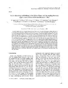
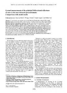
The following indications can be extracted by these distributions: (1) Centaurs belong to the BR group (the larger number) or to the RR taxons, confirming the known color bimodality of that object (Tegler and Romanishin, 1998, Peixinho et al., 2003); the TNOs are distributed in all the taxons, but a larger number of classical objects belongs to the RR taxon. (2) The more distant objects are quite equally subdivided in all the four taxons. (3) The orbital inclinations of the RR TNOs are in general low, confirming the fact that these objects are primordial objects (cold population) with low-inclination orbits, while the high-inclination objects belong to the BB taxon, which seems to be the representative of the “hot” population (Levison and Stern, 2001; Brown, 2001; Doressoundiram et al., 2002; Gomes, 2003; chapter by Doressoundiram et al.). (4) The taxon BR spans the entire range of inclinations, while the taxon IR is characterized by intermediate inclinations (15°–20°). Moreover, in Fig. 4 the distribution of the different taxons within each TNO dynamical class is shown. The bimodality of the Centaurs is evident, the objects classified as
Fig. 4. Distribution of the different taxons within each TNOs’ dynamical class.
IR seem to be concentrate in the resonant and classical dynamical classes, while the RR objects dominate the classical dynamical class. 5.
CONCLUSIONS
We applied two multivariate statistical methods (PC analysis and G-mode analysis) to a sample of 67 TNOs and Centaurs for which a homogeneous set of four colors (B–V, V–R, V–I, and V–J) are available. The results provided a quasicontinuous trend from neutral to very red spectra. The results of the G-mode analysis allowed us to distinguish a finer structure superimposed on this trend, separating four groups of homogeneous objects and one single-class object, confirming the results obtained by Barucci et al. (2005a), which analyzed 51 objects described by the same variables. Analyzing a subsample of 55 objects for which a fifth and a sixth variable (the V–H and V–K colors) are available, the same four groups are confirmed. The significance level (99%) of this grouping is larger that (93%) obtained by Barucci et al. (1987) in classifying a sample of 438 asteroids with the same statistical techniques. This represents a strong indication that colors reveal real differences in the surface nature of the TNOs, probably having originated through their physico-chemical evolution. A classification of TNOs and Centaurs based on their broadband colors has been proposed by Barucci et al. (2005a) using a two-letter designation for each taxon (BB, BR, IR, and RR). Such classification gives a good indication about the resemblances and/or differences among objects. Using the extended version of the G-mode analysisfor those objects with only three colors (B–V, V–R, and V–I), we obtain a preliminary classification of another 66 objects (for a total of 135 objects). Among these, one object remains unclassified, and seven have double classification. The availability of at least a fourth variable (V–J or V–H or V–K) appears to be essential for good statistical applications.
190
The Solar System Beyond Neptune
The behavior of each group with respect to the orbital elements shows that the RR object inclinations are low and those of the BB objects are high, while BR and IR taxons have inclinations spanning the entire inclination range. The Centaurs exhibit a clear bimodality: Most of them belong to the BR or RR taxon (see chapter by Tegler et al.). We can conclude that the multivariate analysis of broadband spectrophotometric data of TNOs provides indications for differences in the surface nature of these objects. The quasicontinuous trend, demonstrated by the principal component analysis, is probably a witness to the possible sequence of the alteration processes undergone by the surface of each object, while the different taxons, obtained with Gmode analysis, indicate the present physico-chemical state of the analyzed objects. It is possible to interpret these results both in terms of evolution of the TNO population and/or in terms of original differences in the composition of the objects. Several scenarios are possible and the lack of fundamental data (albedo, size, mass and size distributions, etc.) make it very difficult to develop a quantitative model describing the history of the TNO population. Here we propose two simple scenarios to provide some clues for interpreting the behavior of the TNOs. In terms of evolution, we can consider that (1) the position of an object along the trend connecting the BB taxon to the RR taxon would indicate the time during which it has been exposed to the different alteration processes (e.g., activity, collisions, cratering, energetic particle bombardment), starting from a given initial state (original or consequence of a resetting event); (2) each taxon represents a different stage in the evolution of the population; (3) the relative number of objects in each group would account for how long that stage has lasted; and (4) the presence of single-object groups may imply the existence of different (cyclic?) evolution paths. In terms of original compositional differences, we can conclude, following Gomes (2003), that the “hot” population is composed by the objects having quite high orbital inclinations and belonging to the BB taxon, while the “cold” indigenous population is that represented by the RR objects, some of which seem to contain very pristine compounds, such as methanol ice. The intermediate BR and IR taxons would represent the results of the aging of the surfaces of the BB and RR objects respectively, due to the exposure to the environmental modifying processes. The energetic particle bombardment of “dirty” icy surfaces induces the formation of dark, redder hydrocarbon coating films, which could be considered to be responsible for the BB → BR transition. A “rain” of micrometeorites over long time intervals may cause the loss of volatiles on the surface of the RR objects and change the characteristics of the overlying ices, which would result in the objects being less red than they were previously: RR → IR. Rejuvenation processes (energetic collisions, degassing activity) can reset most of the surface of an affected object to its initial condition, ac-
tivating a cyclic change in the surface color properties and consequently their classification. REFERENCES Barucci M.A. and Fulchignoni M. (1990) Unified asteroid taxonomy. In Asteroids, Comets and Meteors III (C-I. Lagerkvist et al., eds.), pp. 7–10. Uppsala Universitet, Uppsala. Barucci M. A., Capria M. A., Coradini A., and Fulchignoni M. (1987) Classification of asteroids using G-mode analysis. Icarus, 72, 304–324. Barucci M. A., Doressoundiram A., Tholen D., Fulchignoni M., and Lazzarin M. (1999) Spectrophotometric observations of Edgeworth-Kuiper belt objects. Icarus, 142, 476–481. Barucci M. A., Fulchignoni M., Birlan M., Doressoundiram A., Romon J., and Boehnhardt H. (2001) Analysis of trans-neptunian and Centaur colours: Continuous trend or grouping? Astron. Astrophys., 371, 1150–1154. Barucci M. A., Boehnhardt H., Dotto E., Doressoundiram A., Romon J., Lazzarin M., Fornasier S., de Bergh C., Tozzi G. P., Delsanti A., Hainaut O., Barrera L., Birkle K., Meech K., Ortiz J. L., Sekiguchi T., Thomas N., Watanabe J., West R. M., and Davies J. K. (2002) Visible and near-infrared spectroscopy of the Centaur 32532 (2001 PT13). ESO Large Program on TNOs and Centaurs: First spectroscopy results. Astron. Astrophys., 392, 335. Barucci M. A., Belskaya I. N., Fulchignoni M., and Birlan M. (2005a) Taxonomy of Centaurs and trans-neptunian objects. Astron. J., 130, 1291–1298. Barucci M. A., Cruikshank D. P., Dotto E., Merlin F., Poulet F., Dalle Ore C., Fornasier S., and de Bergh C. (2005b) Is Sedna another Triton? Astron. Astrophys., 439, L1–L4. Bauer J. M., Meech K. J., Fernández Y. R., Pittichova J., Hainaut O. R., Boehnhardt H., and Delsanti A. C. (2003) Physical survey of 24 Centaurs with visible photometry. Icarus, 166, 195– 211. Binzel R. P. and Xu S.(1993) Chips off of asteroid 4 Vesta — Evidence for the parent body of basaltic achondrite meteorites. Science, 260, 186–191. Boehnhardt H., Tozzi G. P., Birkle K., Hainaut O., Sekiguchi T., Vair M., Watanabe J., Rupprecht G., and the FORS Instrument Team (2001) Visible and near-IR observations of transneptunian objects. Results from ESO and Calar Alto Telescopes. Astron. Astrophys., 378, 653–667. Boehnhardt H., Delsanti A., Barucci A., Hainaut O., Doressoundiram A., Lazzarin M., Barrera L., de Bergh C., Birkle K., Dotto E., Meech K., Ortiz J. E., Romon J., Sekiguchi T., Thomas N., Tozzi G. P., Watanabe J., and West R. M. (2002) Astron. Astrophys., 395, 297–303. Brown M. E. (2001) The inclination distribution of the Kuiper belt. Astron. J., 212, 2804–2814. Brown M. E., Trujillo C. A., and Rabinowitz D. L. (2005) Discovery of a planetary-sized object in the scattered Kuiper belt. Astrophys. J. Lett., 635, L97–L100. Bus S. J. and Binzel R. P. (2002) Phase II of the small main-belt asteroid spectroscopic survey. A feature-based taxonomy. Icarus, 158, 146–177. Coradini A., Fulchignoni M., Fanucci O., and Gavrishin A. I. (1977) A Fortran V program for a new statistical technique: The G mode central method. Computers and Geosciences, 3, 85–105.
Fulchignoni et al.: Transneptunian Object Taxonomy
Davies J. K. (2000) Physical characteristics of trans-neptunian objects and Centaurs. In Proceedings of the ESO Workshop on Minor Bodies in the Outer Solar System (A. Fitzsimmons et al., eds.), p. 9. Springer-Verlag, Berlin. Davies J. K., McBride N., and Green S. F. (1997) Optical and infrared photometry of Kuiper belt object 1993SC. Icarus, 125, 61–66. Davies J. K., McBride N., Ellison S. L., Green S. F., and Ballantyne D. R. (1998) Visible and infrared photometry of six Centaurs. Icarus, 134, 213–227. Davies J. K., Green S., McBride N., Muzzerall E., Tholen D. J., Whiteley R. J., Foster M. J., and Hillier J. K. (2000) Visible and infrared photometry of fourteen Kuiper belt objects. Icarus, 146, 253–262. Davies J. K., Tholen D. J., Whiteley R. J., Green S. F., Hillier J. K., Foster M. J., McBride N., Kerr T. H., and Muzzerall E. (2001) The lightcurve and colours of unusual minor planet 1998 WU24. Icarus, 150, 69–77. De Bergh C., Delsanti A., Tozzi G. P., Dotto E., Doressoundiram A., and Barucci M. A. (2005) The surface of the transneptunian object 90482 Orcus. Astron. Astrophys., 437, 1115–1120. Delsanti A. C., Boehnhardt H., Barrera L., Meech K. J., Sekiguchi T., and Hainaut O. R. (2001) BVRI photometry of 27 Kuiper belt objects with ESO/Very Large Telescope. Astron. Astrophys., 380, 347–358. Delsanti A., Hainaut O., Jourdeuil E., Meech K., Boehnhardt H., and Barrera L. (2004) Simultaneous visible-near IR photometric study of Kuiper belt object surfaces with the ESO/Very Large Telescopes. Astron. Astrophys., 417, 1145–1158. Delsanti A., Peixinho N., Boehnhardt H., Barucci M. A., Merlin F., Doressoundiram A., and Davies J. K. (2006) Near-infrared colour properties of Kuiper belt objects and Centaurs: Final results from the ESO large program. Astron. J., 131, 1851– 1863. De Sanctis M. C., Coradini A., and Gavrishin A. (2006) G-mode classification of trans-neptunian objects (abstract). In Lunar and Planetary Science XXXVII, Abstract #1109. Lunar and Planetary Institute, Houston (CD-ROM). Doressoundiram A., Barucci M. A., Romon J., and Veillet C. (2001) Multicolour photometry of trans-neptunian objects. Icarus, 154, 277–286. Doressoundiram A., Peixinho N., de Bergh C., Fornasier S., Thébault P., Barucci M. A., and Veillet C. (2002) The colour distribution in the Edgeworth-Kuiper belt. Astron. J., 124, 2279. Doressoundiram A., Tozzi G. P., Barucci M. A., Boehnhardt H., Fornasier S., and Romon J. (2003) ESO large programme on trans-neptunian objects and Centaurs: Spectroscopic investigation of Centaur 2001 BL41 and TNOs (26181) 1996 GQ21 and (26375) 1999 DE9. Astron. J., 125, 2721–2727. Doressoundiram A., Barucci M. A., Boehnhardt H., Tozzi G. P., Poulet F., de Bergh C., and Peixinho N. (2005a) Spectral characteristics and modeling of the trans-neptunian object (55565) 2002 AW197 and the Centaurs (55576) 2002 GB10 and (83982) 2002 GO9: ESO large program on TNOs and Centaurs. Planet. Space Sci., 53, 1501–1509. Doressoundiram A., Peixinho N., Doucet C., Mousis O., Barucci M. A., Petit J. M., and Veillet C. (2005b) The Meudon Multicolour Survey (2MS) of Centaurs and trans-neptunian objects: Extended dataset and status on the correlations reported. Icarus, 174, 90–104. Doressoundiram A., Peixinho N., Moullet A., Fornasier S., Barucci
191
M. A., Beuzit J. L., and Veillet C. (2007) The Meudon Multicolour Survey (2MS) of Centaurs and transneptunian objects: From visible to infrared colours. Astron. J., in press. Dotto E., Barucci M. A., Boehnhardt H., Romon J., Doressoundiram A., Peixinho N., de Bergh C., and Lazzarin M. (2003) Searching for water ice on 47171 1999 TC36, 1998 SG35, and 2000 QC243: ESO large program on TNOs and centaurs. Icarus, 162, 408–414. Farnham T. L. and Davies J. K. (2003) The rotational and physical properties of the Centaur (32532) 2001 PT13. Icarus, 164, 418– 427. Ferrin Ignacio, Rabinowitz D., Schaefer B., Snyder J., Ellman N., Vicente B., Rengstorf A., Depoy D., Salim S., Andrews P., Bailyn C., Baltay C., Briceno C., Coppi P., Deng M., Emmet W., Oemler A., Sabbey C., Shin J., Sofia S., van Altena W., Vivas K., Abad C., Bongiovanni A., Bruzual G., Della Prugna F., Herrera D., Magris G., Mateu J., Pacheco R., Sánchez Ge., Sánchez Gu., Schenner H., Stock J., Vieira K., Fuenmayor F., Hernandez J., Naranjo O.; Rosenzweig P., Secco C., Spavieri G., Gebhard M., Honeycutt K., Mufson S., Musser J., Pravdo S., Helin E., and Lawrence K. (2001) Discovery of the bright trans-neptunian object 2000 EB173. Astrophys. J. Lett., 548, L243–L247. Fulchignoni M., Birlan M., and Barucci M. A. (2000) The extension of the G-mode asteroid taxonomy. Icarus, 146, 204–212. Fulchignoni M., Delsanti A., Barucci M. A., and Birlan M. (2003) Toward a taxonomy of the Edgeworth-Kuiper objects: A multivariate approach. Earth Moon Planets, 92, 243–250. Gil-Hutton R. and Licandro J. (2001) VR photometry of sixteen Kuiper belt objects. Icarus, 152, 246–250. Gomes R. (2003) Planetary science: Conveyed to the Kuiper belt. Nature, 426, 393–395. Hardorp J. (1980) The Sun among the stars. III — Energy distributions of 16 northern G-type stars and the solar flux calibration. Astron. Astrophys., 91, 221–232. Hartmann W. K., Cruikshank D. P., and Degewij J. (1982) Remote comets and related bodies — VJHK colourimetry and surface materials. Icarus, 52, 377–408. Hainaut O. R., Delahodde C. E., Boehnhardt H., Dotto E., Barucci M. A., Meech K. J., Bauer J. M., West R. M., and Doressoundiram A. (2000) Physical properties of TNO 1996 TO66. Lightcurves and possible cometary activity. Astron. Astrophys., 356, 1076–1088. Jewitt D. C. and Luu J. X. (1998) Optical-infrared spectral diversity in the Kuiper belt. Astron. J., 115, 1667–1670. Jewitt D. C. and Luu J. X. (2001) Colours and spectra of Kuiper belt objects. Astron. J., 122, 2099–2114. Levison H. F. and Stern S. A. (2001) On the size dependence of the inclination distribution of the main Kuiper belt. Astron. J., 121, 1730–1735. Luu J. X. and Jewitt D. C. (1996) Colour diversity among the Centaurs and Kuiper belt objects. Astron. J., 112, 2310. McBride N., Davies J. K., Green S. F., and Foster M. J. (1999) Optical and infrared observations of the Centaur 1997 CU26. Mon. Not. R. Astron. Soc., 306, 799–805. McBride N., Green S. F., Davies J. K., Tholen D. J., Sheppard S. S., Whiteley R. J., and Hillier J. K. (2003) Visible and infrared photometry of Kuiper belt objects: Searching for evidence of trends. Icarus, 161, 501–510. Peixinho N., Doressoundiram A., Delsanti A., Boehnhardt H., Barucci M. A., and Belskaya I. (2003) Reopening the TNOs
192
The Solar System Beyond Neptune
colour controversy: Centaurs bimodality and TNOs unimodality. Astron. Astrophys., 410, L29–L32. Peixinho N., Boehnhardt H., Belskaya I., Doressoundiram A., Barucci M. A., and Delsanti A. (2004) ESO large program on Centaurs and TNOs: Visible colours — final results. Icarus, 170, 153–166. Reyment R. and Joreskog K. G. (1993) Applied Factor Analysis in Natural Sciences. Cambridge Univ., Cambridge. Romanishin W., Tegler S. C., Levine J., and Butler N. (1997) BVR photometry of Centaur objects 1995 GO, 1993 HA2, and 5145 Pholus. Astron. J., 113, 1893–1898. Romon-Martin J., Barucci M. A., de Bergh C., Doressoundiram A., Peixinho N., and Poulet F. (2002) Observations of Centaur 8405 Asbolus: Searching for water ice. Icarus, 160, 59–65. Schaefer B. E. and Rabinowitz D. L. (2002) Photometric light curve for the Kuiper belt object 2000 EB173 on 78 nights. Icarus, 160, 52–58. Sheppard S. S. and Jewitt D. C. (2002) Time-resolved photometry of Kuiper belt objects: Rotations, shapes, and phase functions. Astron. J., 124, 1757–1775. Tedesco E. F., Williams J. G., Matson D. L., Weeder G. J., Gradie J. C., and Lebofsky L. A. (1989) A three-parameter asteroid taxonomy. Astron. J., 97, 580–606. Tedesco E. F., Veeder G. J., Fowler J. W., and Chillemi J. R. (1992) The IRAS Minor Planets Survey. Philips Laboratory Report PLTR-92-2049, Hanscom Air Force Base, Massachusetts. Tegler S. C. and Romanishin W. (1997) The extraordinary colours of trans-neptunian objects 1994 TB and 1993 SC. Icarus, 126, 212–217.
Tegler S. C. and Romanishin W. (1998) Two distinct populations of Kuiper belt objects. Nature, 392, 49. Tegler S. C. and Romanishin W. (2000) Extremely red Kuiper belt objects in near-circular orbits beyond 40 AU. Nature, 407, 979– 981. Tegler S. C. and Romanishin W. (2003) Resolution of the Kuiper belt object colour controversy: Two distinct colour populations. Icarus, 161, 181–191. Tegler S. C., Romanishin W., and Consolmagno S. J. (2003) Colour patterns in the Kuiper belt: A possible primordial origin. Astrophys. J. Lett., 599, L49–L52. Tholen D. J and Barucci M. A. (1989) Asteroid taxonomy. In Asteroids II (R. Binzel et al., eds.), pp. 298–315. Univ. of Arizona, Tucson. Trujillo C. A. and Brown M. E. (2002) A correlation between inclination and colour in the classical Kuiper belt. Astrophys. J. Lett., 566, L125–L128. Trujillo C. A., Brown M. E., Barcume K. M., Schaller E. L., and Rabinowitz D. L. (2007) The surface of 2003 EL61 in the nearinfrared. Astron. J., 665, 1172. Wood H. J. and Kuiper G. P. (1963) Photometric studies of asteroids. Astron. J., 137, 1279. Zellner B., Tholen D. J., and Tedesco E. F. (1985) The eight-colour asteroid survey — Results for 589 minor planets. Icarus, 61, 355–416.