KSME International Journal, Iiol. 18 No. 6, pp. 879 ~ 894, 2004
879
(Invited Review Artiele~
Sizing of Spray Particles Using Image Processing Technique Sang Yong Lee*, Yu Dong Kim Department o f Mechanical Engineering, Korea Advanced Institute o f Science and Technology, Science Town, Daejeon 305-701, Korea
The image processing technique is simple and, in principle, can handle particles with various shapes since it is based on direct visualization. Moreover, a wide measurement area can be covered with appropriate optical arrangement. In the present paper, various techniques of image processing for sizing and counting particles are reviewed and recent developments are introduced. Two major subjects are discussed in detail : identification of particles (i.e., boundary detection and pattern recognition) and determination of in-focus criteria. Finally, an overall procedure for image processing of spray particles is suggested. Key W o r d s : I m a g e Processing, Particle Size Measurement, Spray
1. Introduction Various optical techniques have been being used as the non-intrusive method to size drops and particles, such as the phase-Doppler particle analysis ( P D P A ) , light scattering method and the image processing technique (Chigier, 1983). The P D P A technique is based on processing of Doppler effect of the Mie scattering signals coming from the particles passing through a measuring volume. Thereby, simultaneous measurement of size and velocity of individual particles is available. Though the fiber optics are adopted in the system, however, the optical alignment is still cumbersome and the price of the equipment is rather expensive. Other technique widely being used is the light scattering method based on the Fraunhofer diffraction theory (Swithenbank et al., 1977). This technique is relatively simple and also has an advantage of easy alignment. However, this has disadvantages * Corresponding Author, E-mail :
[email protected] TEL : -t-82-42-869-3026; FAX : -t-82-42-869-8207 Department of Mechanical Engineering, Korea Advanced Institute of Science and Technology, Science Town, Daejeon 305-701, Korea. (Manuscript Received February 3, 2004; Revised April 21, 2004)
of multiple scattering and vignetting effects (Wild and Swithenbank, 1986) that have to be corrected empirically. The above two techniques are deducing the particle size information from the optical signals scattered from individual or group of particles in the measuring volume assuming that the particles are all spheres. Thus, basically, only the spherical particles should be processed with those techniques for accurate measurement (Malot and Blaisot, 2000). On the other hand, in principle, various non-spherical particles can be processed through the image processing technique because it is based on direct visualization, and wide application is possible. Moreover, the measurement accuracy of the image processing techniques is relatively insensitive to the optical properties of the particles compared to the other techniques, and the optical alignment is much easier (Lecuona et al., 2000). However, the image processing technique also has shortcomings: a number of image frames have to be processed to get the statistically meaningful distributions for a control volume because the data acquisition rate is usually low (i.e., number of spray particles contained in an image frame is usually small) (Nishino et al., 2000). Also, the accuracy of the results strongly depends on the depth of field
880
Sang Yong Lee and Yu Dong Kim
criterion (Chigier, 1991: Nishino et al., 2000). The ultimate goal of the image processing research is to identify the objects of interest (spray particles in the present case) and to measure their sizes. The in-tbcus criteria should be provided to decide whether to count or not, and the boundaries of objects should be detected and identified effectively. The particle identification process includes determination of the threshold level for boundary detection, separation of primary particles from their agglomerated or overlapped images, and treatment of non-spherical particles. Finally, once the particles are identified, those are sized and counted to give the size distribution. In the present paper, various image-processing techniques are discussed and compared to each other to find out their merits and demerits in detail ; and then recent developments to improve the measurement accuracy and efficiency of these techniques are briefly introduced.
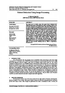
2. Fundamental System Hardware Basically, the system hardware for image processing consists of a light source, a camera and a computer with the accessories as shown in Fig. I. In most cases, the camera, object and the light source are placed in line with backward illumination. However, for image processing of fluorescent particles, the technique of side illumination with a laser sheet is often used. An instantaneous light source (flash strobolight) is used to capture the frozen images of spray particles in
i z
R~vn i gI
/o~o\
Camera Unit
F ~ n t r oBoard l
Grabber
~
P Light Source
Control &Image Processing Unit
Fig. 1 Hardware setup of image processing technique (Kim, 2000)
the flow field. Thus the flashing duration should be as short as possible to capture small or highspeed particles. For the camera system, traditional film cameras may be used ; however C C D (Charge-Coupled Device) cameras are widely being adopted to eliminate the manual scanning process for digitization. Computers are equipped with a time control board and a frame grabber to synchronize signals and to store the captured images. The computer also processes the stored images to get the final results.
3. In-Focus Criterion The depth-of-field effect is one of the major factors influencing the measurement accuracy. There are two possible error sources concerned with the depth-of-field effect (Chigier, 1991; Nishino et al., 2000). One is the ambiguity in defining the boundaries of the particles that are placed outside the focal plane. The ambiguity increases as the particles are located farther from the focal plane. Thus, one should judge whether to count or not from the degree of ambiguity. This has been studied in some detail by Kim and Kim (1994) and will be discussed later. Another is the dependency of the depth of field on the particle size. As the particle size becomes smaller, the depth of field drastically decreases, and hence, small particles in a pre-determined measuring volume are more likely to be missed in counting. As a result, the particle size distribution is biased toward a larger size region (Oberdier, 1984; Koh et al., 2001). Therefore there should be a way to correct this effect by adjusting the depth of field corresponding to the particle size, which will also be introduced later. As an indicator of the in-focus criteria, either of the following concepts may be adopted : the gray-level gradient at the particle boundaries (Fantini et al., 1990 ; Lecuona et al., 2000) or the contrast value between the particles and the background of the image frame (Kim and Kim, 1994: Lebrun et al., 1996; Malot and Blaisot, 2000). Later, Koh et al. (2001) proposed appropriate size ranges for each concept.
Sizing of Spray Particles Using Image Processing Technique 3.1 Criterion by gray-level gradient As a particle is located farther from the focal plane, the gray level at the edge of the particle image changes more gradually as shown in Fig. 2 (Koh et al., 2001), and the gray-level gradient can be used to express the degree of focus of the particles (Ramshaw, 1968; Fantini et al., 1990). In this figure, z denotes the axial distance from the focal plane with the positive value being the direction toward the CCD camera as shown in Fig. 1. Figure 3 illustrates typical gray-level profiles for an in-focus and an out-of-focus particle (Fantini et al., 1990). The gray-level gradient of the focused particle is steeper than that of the unfocused one. Two gray levels, /2 and A, defining a "halo" around the particle can be identified, which correspond to diameters d2 and d3, respectively. Then the width of the halo (Ad/2) equivalent to (d3-d2)/2 can be used as an index of in-focus criteria (Fantini et al., 1990). That is, if Ad/2 is larger than H ( d ) , a function of
z--
--400urn
--300/zm
z = 0 p m (focal plane)
100 izm
--200 ,tan
-- I00 ,urn
200 ,um
300 A,m
Fig. 2 Change of particle images with distance from the local plane (300-micron particle)
the particle diameter obtained through the calibration process, the corresponding particle is eliminated in counting. Figure 4 exhibits the calibration results for various particle diameters ranging from 30 microns to 340 microns. Thus, by using the calibration result with the halo width, actual particle diameters could be predicted from the measured values. Lecuona et al.(2000) also employed the concept of gray-level gradient to eliminate the unfocused particles in simultaneous measurement of particle sizes and velocities. There, they defined the in-focus parameter as
inf=K
~
iiiiiii
gradcomp----
(1)
(2)
Imax--Iback dp
Here, K = 0 . 0 1 and dp represents the particle diameter. Also, /max and Ibach are the maximum and background gray levels, respectively. The gray level gradient at the edge of the particles, gradmax, is obtained from the Sobel operators (Gonzalez and Woods, 1993). This parameter is insensitive to the local brightness of the image frame. Figure 5 shows variations of inf with the distance from the focal plane for different aperture numbers (F) and particle (glass sphere) diameters ranging between 0.5 mm and 3 mm. 3O
+••.
d
t~m)
x
340
.4o
204 141
•
113
::
Q,
[
//
,o
2Hal°~" ~ ~ ~ a r m i n g co-ordinate O
Fig. 3
gradmax gra dcomp
with the following definition:
iiiiiii
f
881
ore~.~. ~ - ~ O u t - o f-focus In-focus Drop image intensity profiles (Fantini et al., 1990)
2
t -1
I 0
i 1
Distance from in-focus plane (mm) Fig. 4
Halo width variation with position in field (Fantini et al., 1990)
Sang Yong Lee and Yu Dong Kirn
882
$
convolution :
,o F- 16 7
a ~ . ~ ~
I(r) =A(r)
- - ~ - - F ~ 11
* h(r)
(3)
where A ( r ) = l - c i r c ( r / d ) and d is the geometric image radius. The value of c i r c ( r / d ) is unity for r ~ d and zero elsewhere. Also 8 h(r) =~-exp
[ ~
.
-
-
-
.
_
I":' :----:':'7 ""
o.!,;--'- ~"
':
-5
,
" 0
"'~;:.7"-
' -,r .... ':, ~
"-
''-:.
10
--8r 2 ( ~ )
(4)
which is the Gaussian point spread function (PSF) and a represents the spatial parameter of PSF. The value of a increases as the distance from the focal plane increases. The image contrast is defined as
Distance fromthe objectplane [mm*10"1] C - I(oo) - I ( 0 ) I(~) +I(0)
Fig. 5 Variation of i n f with respect to axial distance from object plane (Lecuona et al., 2000) Based on this calibration curve, critical value of i n f for each size can be determined by imposing a proper value of the depth of field, and the particles with smaller i n f are considered as out of focus.
3.2
Criterion by value of contrast
Kim and Kim (1994) performed an extensive study on the image processing technique to size liquid drops less than 30 microns discharged from a fuel injector. Their study includes the determination of the threshold gray level and infocus criterion. They introduced the concept of the normalized value of contrast ( V C ) to determine if the drops are in focus or not. With this concept, the depth-of-field correction has been performed for each size of drops. This criterion is known to be effective for sizing small drops, and will be discussed later along with the work by Koh et al.(2001). In the work of Lebrun et a1.(1996), o u t - o f focus images are deconvoluted with the assumption of a Gaussian point-spread function, where the spatial parameters increases with the distance from the focal plane. Similar approach has been performed independently by Malot and Blaisot (2000). The intensity (gray level) distribution on CCD plane may be expressed with the following
(5)
where I ( c o ) and / ( 0 ) are the intensities at r - - ~ ov and at the image center, respectively. The image contrast can be expressed in terms of particle diameter (d) and the degree of o u t - o f focus (o'). In their case, the gray-level threshold was set to 1 = 0 . 5 5 { 1 ( o o ) - - I ( 0 ) } + I ( 0 ) . Thereby, through the calibration process with the particles of known sizes, a relationship between the true value and the measured one could be obtained. According to Lebrun et a1.(1996) and Malot and Blaisot (2000), the dependency of the ratio between the measured and true radii on the image contrast (C) becomes weaker as the value of C approaches unity. This implies that this criterion is not effective to judge the degree of focus for large particles.
3.3
Unified in-focus criterion
From the previous discussions, it can be realized that the criterion of gray-level gradient is mostly suitable to large particles whereas the criterion of contrast value is for small particles. In this view, Koh et al.(2001) suggested to adopt both criteria by introducing the appropriate particle-size ranges for each case. F o r the particles smaller than 30 microns, based on their optical arrangement, the normalized value of contrast (Kim and Kim, 1994) defined as
VC = GEe-- GoM G~B
(6)
Sizing of Spray Particles Using Image Processing Technique was used as an index of the in-focus criterion. Here, GLB and GoM represent the local background and the object minimum gray levels, respectively, as shown in Fig. 6. Figure 7 shows the variation of VC with the distance from the focal plane for particle size range of 8-300 microns. The VC value becomes the largest at or near the focal plane and decreases as becomes unfocused. However, the variation appears gradual with the larger particles. This implies that VC is no longer effective as the index of the degree of focus. In other words, for a large outof-focus particle, the radius (d/2) is always greater than the boundary width (w), and the value of Gora remains unchanged. For particles larger than 30 microns, the concept of the gradient indicator (G I) was introduced as an index of the in-focus criterion, defined as ,
2i BackFlr°und
i
! j _ _ ~ .....
CI=
883
IVGI
(7)
which has the similar concept with i n f (Eq. (1)) of Lecuona et a1.(2000). Here, from Fig. 8, the gray level gradient is
lVG(x, y) -- LF \{ ac a ~ -?/ - r,k /~ )ac
cgG_ (C~+2G6+C~) -- ( G ~ + 2 G 4 + Gv) 3x
8Ax (9)
3G _ (C-v+2C-8+ C-9) - ( G I + 2 G z + G a ) 3y 8Ay As shown in Fig. 9, the values of GI show the maximums at or near the focal plane and decrease as away from the focal plane. Thus GI can be used as an index of the degree of focus as well. Figure l0 shows the depth of field variation with
G1 :
(8)
and, for pixel #5, the gray level gradients in x and y directions can be expressed with the Sobel operators as follows;
i i
w
]
,
Y
G3
G2
G4 ~
G6
Dark k e v e ? L ' ~
Fig. 6
Gray level changes with different particle size (Koh et al., 2001)
G7 G8 G9 ;x
Fig. 8
Numbering of the pixels to express gray level gradient at pixel #5
1.00.9-
~3001arn
~0.8.
.~ 0.7.
,
lro~
/..
/ s
~
0.6
\
\
8 0.6.
.
0.5
~ 0.s.
O.4
~ 0,4-
~
-
=
:tt'~
-
~ 0.3. ~ 0.2,
E
~ 0.1Z 0.0 -2.5
01 -2.0
-1.5
-1.0
-0.5
0.0
0.5
1.0
1.5
-2.5
Distance from Focal Plane, z (mm)
Fig. 7
Variation of normalized value of contrast (VC) with distance from focal plane for each particle size (Koh et al., 2001)
-2 0
-1 5
-1.0
-0.5
00
05
1.0
Distance from Focal Plane, z ( m m )
Fig. 9
Variation of gradient indicator (G1) with distance from focal plane for each particle size (Koh et al., 2001)
884
Sang Yong Lee and Yu Dong Kim
13-
•
+10%
•
• •
_ __
Spot Diameter
121.1 1.0: E
0.95
E ~" 0.8$ o.~ "~ 0.6i
/:'
~'~-10% ~rOD
E ~- 0,5 121 0.4
t::
Di~lr~Aeter
0.:1 i ~ ! - ~VC GI
0.2
•
•
,I
.
i
5o
. . . .
i
~oo
. . . .
r
. . . .
15o
•
VC-applicable
•
GI-applicable i
2oo
. . . .
i
250
. . . .
i
300
Particle Size(pm)
Fig, 11 Sample Image of Glass Sphere (Saylor and Jones, 2002)
Fig. tO Variation of depth of field with particle size (Koh et al., 2001)
the particle size ranging from 10 to 300 microns, mostly covers the fuel spray drops. Here, by introducing two different indices, VC and G1, the measurement accuracy could be maintained below ten percent. The relationship between the depth of field and the particle size is very useful because it can be utilized in the process of the depth-of-field correction for a fixed measuring volume (Kim and Kim, 1994).
3.4
Other related works
The previous methods introduced in the earlier sections are the techniques generally used to resolve the out-of-focus problem. However, there are some other works related to determination of the in-focus criteria (Nishino et al., 2000 : Saylor and Jones, 2002). Saylor and Jones (2002) developed an imageprocessing algorithm to improve the performance of the rain imaging system (RIS) for raindrop size measurement. In order to secure a sufficient number of drops in a single image frame, the depth of field should be increased. At the same time, increasing of the depth of field causes the increase of the measurement error since the sizes of the unfocused particles appears to be different from the true values. Therefore, in their work, a method to increase the depth of field was proposed without losing the measurement accuracy. With the backward illumination, a bright spot is observed at the center portion of the transparent particles as shown in Fig. I1. The bright
spot is the image of the light source, as seen through the drop, and appears sharp when the drop is at the focal plane. (The light source used in their experiment has a rectangular shape.) As the drop is away from the focal plane, the spot becomes ambiguous. Saylor and Jones (2002) showed that, by using glass spheres, parameter a defined as the ratio between the spot diameter and the drop diameter (Fig. I1) depends solely on the distance from the focal plane. However, the sizes of the glass spheres tested were ranging from 4 mm to 10 mm and only applicable to large transparent particles such as raindrops. Lecuona et a1.(2000) also have noted that the sharpness of the image may be used as an indicator of degree of focus. Nishino et al.(2000) used two CCD cameras to obtain stereo images of particles for simultaneous measurement of size and three velocity components of particles in dispersed two-phase flow. The technique developed was capable of sizing 10-500 microns. As a part of their experiment, the resolution of the depth-of-field effect in particle sizing was considered. They noted that the diameters of small particles (smaller than 40 microns) tend to be overestimated while those of the larger ones (larger than 100 micros) show the opposite trend.
4. P a r t i c l e
Identification
The shape and size information of the particles in an image frame is obtained through the particle identification process. The general proce-
Sizing of Spray Particles Using Image Processing Technique dure is to separate out the particles from the background of the image frame by using the boundary detection algorithms, and then the size and shape of the binary images of the particles are measured and recognized by using the pattern recognition algorithms. The particle diameter can be deduced once the number of pixels occupied by the particle image and the scale factor (length/pixel) of the optical system are given. The details are discussed in the following sections.
885
1.~000 Threshold 12006
l.eveJ ~ 8 0 % o f I n t e r s e c t i o n Gray Level
\
~ 9000 g ta_
6000
b
3000
0 52
64
96
128 lfi0 Gray Level
19~'
Boundary detection
GLr -- GLB
(Kim,
2000)
There are two indicators mainly used to detect the particle boundaries : gray-level threshold and gray-level gradient. Gray-level threshold is the indicator most widely considered in detecting the particle boundaries since it is simple to use (Otsu, 1979; Fantini et al., 1990; Lee et al., 1991 ; Kim and Kim, 1994 ; Lebrun et al., 1996 ; Kim et al., 1999 ; Kim, 2000; Malot and Blaisot, 2000; Sudheer and Panda, 2000; Koh et al., 2001 ; Saylor and Jones, 2002). For a given image frame, the portions with the gray level lower than a threshold value are counted as particles and the rest parts are considered as the background. In this case, the number of the detected particles as well as their sizes depends on the threshold level, and care should be taken to decide this value. There are two different ways to determine the threshold gray level; taking an appropriate value simply between the gray levels of each particle and the background (Kim and Kim, 1994 ; Lebrun et al., 1996; Kim et al., 1999; Kim, 2000; Malot and Blaisot, 2000; Koh et al., 2001), or obtaining from the gray-level histogram of the image frames (Otsu, 1979 ; Fantini et al., 1990 ; Lee et al., 1991 ; Kim, 2000 ; Sudheer and Panda, 2000 ; Saylor and Jones, 2002). As a simple thresholding criterion, Kim and Kim (1994), Kim et a1.(1999) and Koh et al. (2001) have taken the threshold value ( T ) , defined as (Fig. 6)
T = G o u - GLB
256
Fig. 12 Typical histogram of a spray image and determination of threshold level
4.1
224
( 1O)
to be 0.5. However, the value strongly depends on the quality of the image frames and Lebrun et al. (1996) and Malot and Blaisot (2000) suggested l - Z to be 0.55 and 0.61, respectively, through their own calibration process. The method using the gray-level histogram has been adopted in the works of Otsu (1979), Lee et a1.(1991), Kim (2000) and Sudheer and Panda (2000). Figure 12 shows a typical graylevel histogram of a spray image, in which the gray-level range near the peak value corresponds to the background. However, the gray levels of the particles are mostly zero and, though not shown in the figure, there is a sharp local peak coincides with the ordinate of this plot. Therefore, Lee et al. (1991) have taken one-half of the gray level corresponding to the peak of the histogram as the threshold value. On the other hand, as the threshold level to identify the particles, Kim (2000) took the 80%-value of the intersection of the abscissa and the tangential line at the steepest gradient of the histogram as illustrated in Fig. 12. More sophisticated approach has been attempted by Otsu (1979) and adopted later by Sudheer and Panda (2000). They determined the threshold value based on the zeroth and the first order cumulative momentums from the gray-level histogram. To help illustrating this method, a schematic of the graylevel histogram was given in Fig. 13 along with the important parameters. Here, let #o and /11 represent the mean gray levels (first-order cumu-
Sang Yong Lee and Yu Dong Kim
886 / 11¢/
Dividing Line (Threshold Level) /J1
>.
wl t~.
Po
50,
°;, ~xel Position
(a)
I
(b)
Gray Level Fig. 13
Illustration of the method of Otsu (1979) for gray-level threshold O
lative moments) of each gray-level group of the histogram, respectively, divided by a vertical line in the figure. Similarly, let w0 and a~l be the numbers of the pixels belong to each graylevel group (i.e., the zeroth-order cumulative moments). Then the line dividing the gray-level group in Fig. 13 would represent the optimal threshold if the value of a)0col(~--/zx) 2 is the maximum. It has an advantage of avoiding consideration of the local valleys of the histogram by using the integrated values. However, it should be mentioned that the threshold level determined by this method varies with the change of the number concentration of the particles contained in an image frame even though the size distribution remains the same. Gray-level gradient method is based on the assumption that the gray-level variation is the steepest at the particle boundaries as illustrated in Fig. 14. Figure 14(a) is the original image of a particle, while Fig. 14(c) is its converted image in the plane of the gray-level gradient. Figs. 14 (b) and (d) are the plots of the gray level and its gradient corresponding to Figs. 14(a) and (c), respectively. The brightest part of the ring-shaped image in Fig. 14(c) corresponds to the steepest gradient of the gray level. Kim and Lee (2002) used this method in identifying the primary particles from the images of heavily overlapped particles. From the plot of gray-level gradient, as exemplified by Fig. 14(d), an appropriate threshold value was imposed to recognize the particle boundary. Here, there may be more than one pixel having the gradient greater than this threshold
O 0
• 0
Pixel Pos~lo~
(c) Fig. 14
(d) Sample image and its gray level gradient
value ; and they went through the boundary thinning process down to the 1-pixel thickness. On the other hand, Nishino et a1.(2000) traced the maximum gradient points along the edge of the particle boundary by curve fitting. 4.2
Pattern
recognition
and s i z e m e a s u r e -
ment
Once the particle boundaries are sought and the binary images are obtained, the shape and size of the particles can be identified and measured. The shapes of the particles are either spherical (circular) or non-spherical (non-circular). Besides, the separation of the overlapped particles is performed in this stage. The common method to measure the particle size is finding of the equivalent diameter of a circle having the same projected area regardless of its original shape (Fantini et al., 1990 ; Lebrun et al., 1996; Sudheer and Panda, 2000). For spherical particles, the radius can be obtained from the mean distance from the boundary pixels to the mass center as follows : • s = ~ I ~/(xh--x~) Radm k=l
z + (yk--yc) 2
(ll)
Sizing of Spray Particles Using Image Processing Technique
Center(xc,
1 ~v 1 yc)=(~k~__,Xk, ~,~__,.Yh) (12)
887
shown in Fig. 15(b). An image processing method based on the correlation analysis in the frequency (Fourier) domain has been reported by Cruvinel et al. (1999). First, reference (standard) images of a particle with various sizes are prepared. Then the particles in the image frames of interest were sought by matching their patterns with the reference images using the Fourier transform process. Figure 16 illustrates this technique in detail. Figure 16(a) shows an input image treated with a threshold area processing. Figure 16(b) shows the standard image of a particle to be recognized from the input image. Figures 16(c) and (d) are the Fourier spectra of the input image and the standard image. Figure 16(e) is the correlation map of the spectra obtained through convolution, where the particle of interest shows the highest correlation (i.e., the brightest spot appears), and Fig. 16(f) is the final result recognizing the particle image having the same radius with the standard image. F o r overlapped particle images, Kim and Lee (1990), Lecuona et al.(2000) and Malot and Blaisot (2000) simply eliminated them since they are considered either odd-shaped foreign materials or erroneously detected. This concept is acceptable only when the drop area fraction ( D A F ) of the image frame is low since the chances of the particle overlap are usually small. Zhang and lshii (1995) and Shen et al.(2001) reported their works on the treatment of the overlapped particles, but the details are not given
Here, N , xk and yk denote the number of pixels at the image boundary and their x - y locations in the plane, respectively. The result is mostly acceptable because the particles are spherical or nearly spherical. However, it gives inaccurate results for the partly detected or overlapped images of particles. To overcome this difficulty, Kim et a1.(1999) proposed to find the circumcenter of the particle image instead of the mass center. Figure 15 illustrates the concept of this method. Once points A , B, and C are selected from the boundary pixels, a triangle A B C is determined as in Fig. 15(a). Then the circumcenter (point O) of this triangle is found at the cross point of the perpendicular lines (OP, OQ and OR) bisecting each side. When there are more than three data points at the particle boundary, a circle that best fits those points should be found. That is, with N data points, N ( N - I ) ( N - 2 ) / 6 triangles and their circumcenters are found, and from the arithmetic mean values of the center locations and the radii of the circles, a circle that best fits all data points can be determined. Here, it should be noted that the three data points should be distant from each other to avoid an erroneous result as illustrated by adjacent points D, E and F in Fig. 15 (a), and the details on this technique are explained in the work of Kim et a1.(1999). The circumcenterbased concept has the advantage when only the partial data points are available for analysis as •,l(x. y0
Mass-center-basedcircle
/
P data points
C (x3,YO 2)
Circumcenter-basedcircle (a) Fig. 15
(b) Detection of the circumcenter (Kim et al., 1999)
i~ lrmge boundary
888
S a n g Y o n g Lee a n d Yu D o n g K i m
,
,
-; ;-~ea, :,. o u r
in their paper. Thus, in the present review, the methods of the particle separation using the Hough transform (Kruis et al., 1994; Crida and de Jager, 1997; Kim and Lee, 2002), the boundary curvature detection (Kim et al., 2001), and the convex-hull method (Kim et al., 1999) are discussed. Using of the Hough transform is very effective way to handle the heavily overlapped particles. Basically, the primary particles are separated out from the agglomerated image, and at the same time, each particle size can be estimated. Figure 17 illustrates the principle of the Hough transform process to identify a circle image. The rectangular symbols in Fig. 17(a) (except for pixels a, e and f ) are the boundary pixels of a particle to be identified. Circle A is the true circle with radius R and the center is located at a ( X , Y ) . With the assumed radius (R) of circle A , its center should exist somewhere at distance R from the boundary pixels. For example, the center of circle A should be a peripheral point of circle B (b-centered circle) with radius R. At the same time, the center of circle A should be a peripheral point of circles C and D, corresponding to boundary pixels c and d. If the circle drawing is repeated along the boundary pixels of circle A, pixel a will have the highest frequency of pass by the circles. In other words, pixel a
"e •
• "".o."
(a)
(b)
(c)
(d)
L
O
¸
(e) (f) Fig. 16 Result of drop identification (Cruvinel et al., 1999)
f;
,.k. }~ (
i ~, -
~)()tznda W',' I)I'